Lecture 2: Numerical Methods

Jan Benáček

Institute for Physics and Astronomy, University of Potsdam

October 26, 2023

Table of contents

• Lecture overview
• 1 Plasma properties
• 2 Plasma simulations
• 3 Hands-on
• 4 Bibiography and references
• 5 Introduction to numerical methods
• 6 ODEs
• 7 PDEs
• 8 References

Lecture overview

Table of Contents 1/2

• 19.10. Introduction + numerical methods summary
• 26.10. Numerical methods for differential equations - lecture + hands-on
• 02.11. Test particle approach — lecture
• 09.11. Test particle approach — hands-on
• 16.11. PIC method — lecture
• 23.11. PIC method — hands-on
• 30.11. Fluid and MHD — lecture

Table of Contents 2/2

• 07.12. Fluid and MHD — hands-on
• 14.12. Radiative transfer — lecture
• 11.01. Radiative transfer — hands-on
• 18.01. HPC computing — lecture + hands-on
• 25.01. Advanced — Smooth particle hydrodynamics method — lecture
• 01.02. Advanced — Hybrid, Gyrokinetics — lecture
• 08.02. Advanced — Vlasov and Linear Vlasov dispersion solvers — lecture

1 Plasma properties

1.1 Plasma parameters

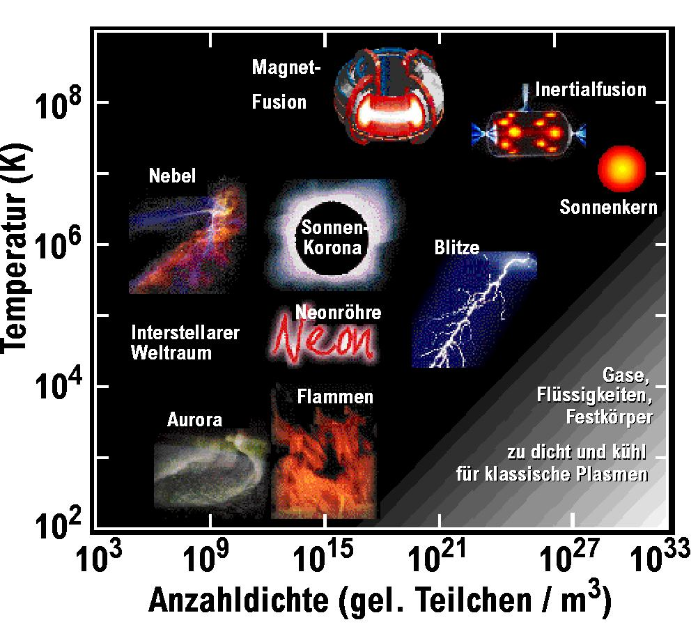
• Temperature
• Number density
• Magnetic field (not in the figure)
  
  
• Cold plasmas
• Hot plasmas

1.2 Collisions in plasmas

• Plasmas can be partially or fully ionized.
• Scattering is different: collisions among and with neutrals: large angle scattering.
• Charged particles: smooth small angle scattering only.
• Collisions enforce thermal equilibrium.

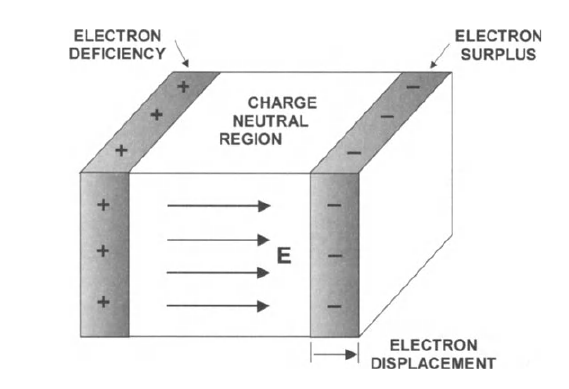
1.3 Length scales: Debye length

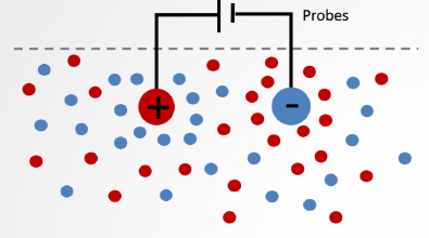
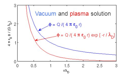
• The Coulomb potential of each particle is shielded by other charges \[\phi_D=\frac{q}{4\pi\epsilon_0 r}\exp\left(-r/\lambda_{De}\right).\]
• The electrostatic potential is screened out on distances larger than the Debye length \[ \lambda_{De} = \sqrt{\frac{\epsilon_0 k_B T_e}{n_e e^2}}. \]
• The plasma is quasi-neutral only for distances \(L\gg \lambda_{De}\).
• At sub-Debye length scales, charge separation occurs.
• An ideal plasma must have a sufficient number of particles in a Debye sphere to enforce their collective behavior. Plasma parameter \[ N_D=n_e \left( \frac{4}{3}\pi \right)\lambda_{De}^3 \gg 1. \]

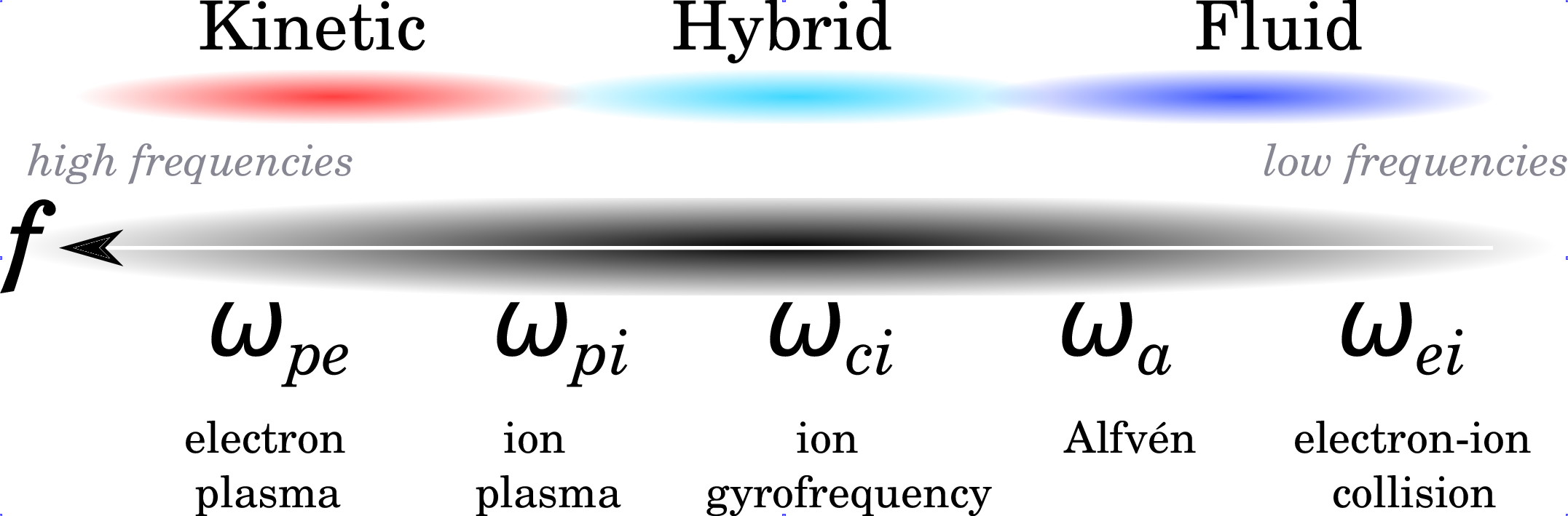
1.4 Time scales: Plasma frequency

• Plasma frequency \[ \omega_{pe}=\sqrt{\frac{n_e e^2}{\epsilon_0 m_e}}. \]
• Typical response of electrons to restore quasineutrality when disturbed by external forces.
• Note that \[ \omega_{pe}= \frac{v_{th,e}}{\lambda_{De}}=\frac{\sqrt{\frac{k_BT_e}{m_e}}}{\lambda_{De}}. \]
• Collective behaviour

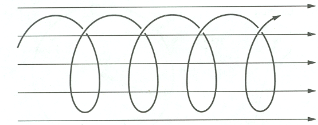
1.5 Time scales: Magnetic field and gyromotion

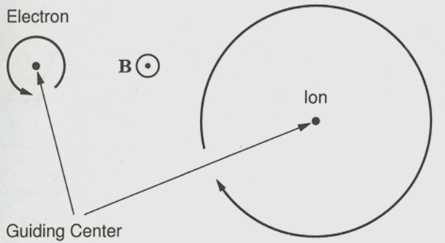
• Single particle motion and Lorentz force \[ m\frac{d\vec{v}}{dt}=q\vec{v}\times\vec{B} \]
• Gyro/cyclotron/Larmor-frequency \[ \Omega_c=\frac{qB}{m} \]
• Gyro/Larmor-radius \[ \rho=\frac{|v_{\perp}|}{\Omega_c}=\frac{m|v_{\perp}|}{|q|B} \] (usually \(|v_{\perp}|=v_{th}\)).
• Ratio of thermal to magnetic pressure. Plasma-\(\beta\) \[ \frac{nk_BT}{\frac{B^2}{2\mu_0}} \propto \left(\frac{\omega_{pe}}{\Omega_{ce}}\right)^2\left(\frac{v_{th}}{c}\right)^2. \]

1.6 Other relevant parameters

• Thermal speed \[ v_{th} = \sqrt{\frac{k_bT}{m}} \]
• Alfvén speed \[ V_A = \frac{B}{\sqrt{\mu_0 n m_i}} \]
• Ion skin depth/inertial length \[ d_i = \frac{c}{\omega_{pi}} = \frac{V_{A}}{\Omega_{ci}} \]

1.7 Plasma parameters

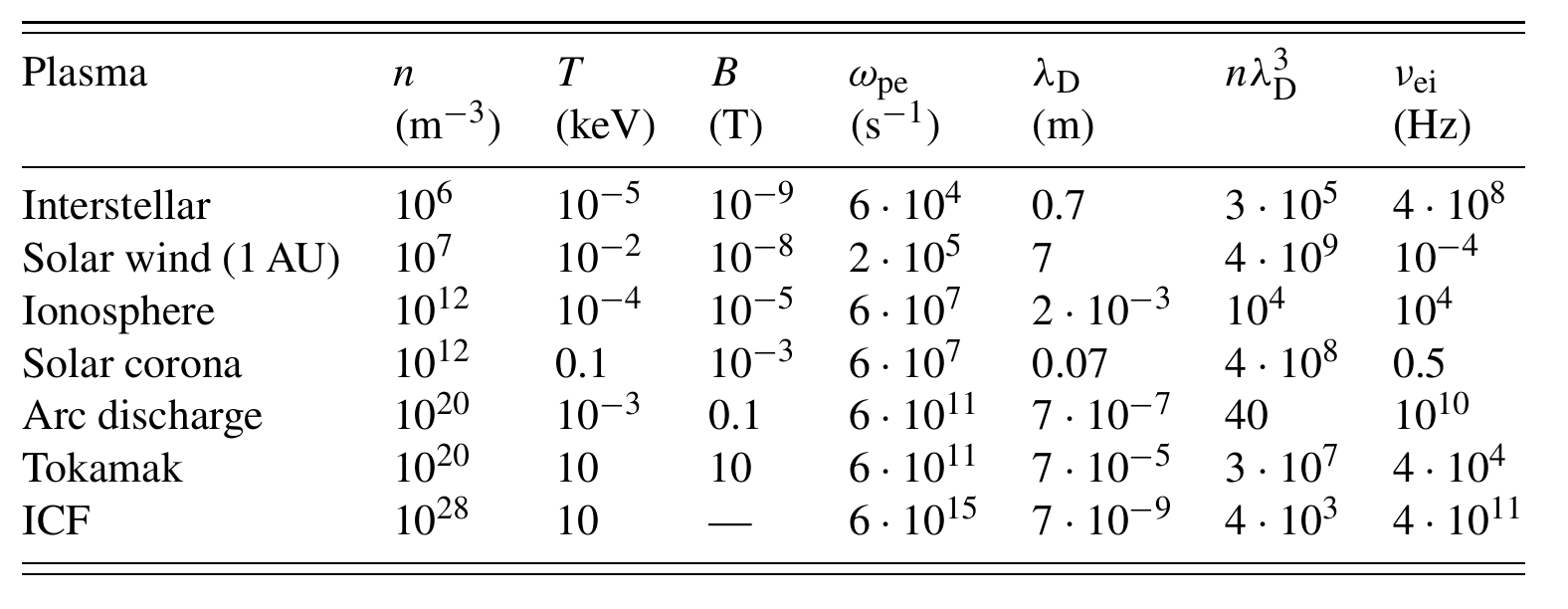
ICF = Inertial Confinement Fusion

(Boyd and Sanderson 2003)

1.8 Your turn

1. Which main parameters can be used to describe a plasma?
2. Select parameter(s) and discuss its physical and intuitive meaning.
3. What are approximative values of the plasma parameters in your favorite plasma environment?

2 Plasma simulations

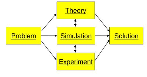
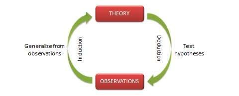
2.1 The role of simulations in science

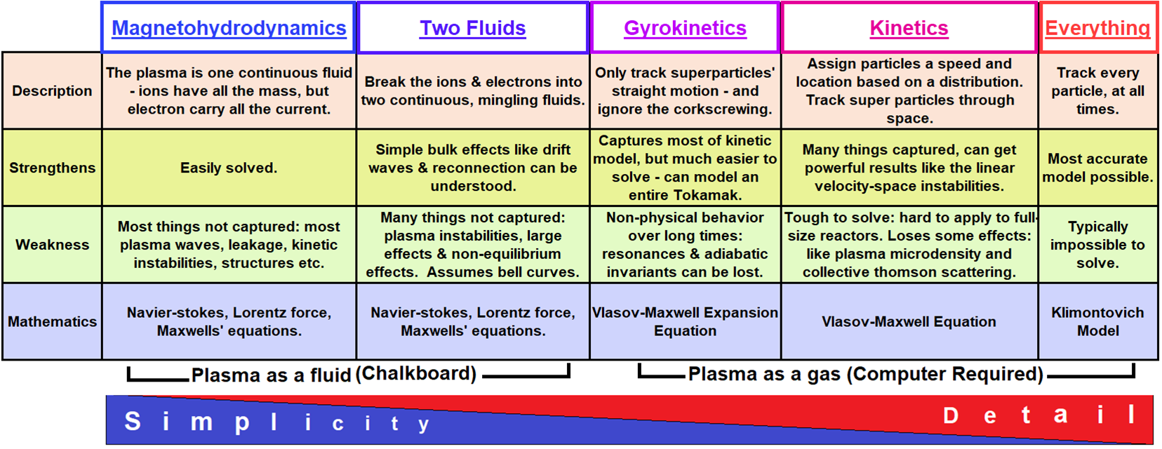
2.2 Hierarchy of plasma physics models

Kinetic description

Microscopic properties, it uses the velocity distribution function \(f(\vec{x}, \vec{v}, t)\).

Fluid description

Uses a few macroscopic quantities, averages of the distribution function (mean velocity \(v(\vec{x},t)\), pressure/temperature). Valid for exact or near thermodynamic equilibrium.

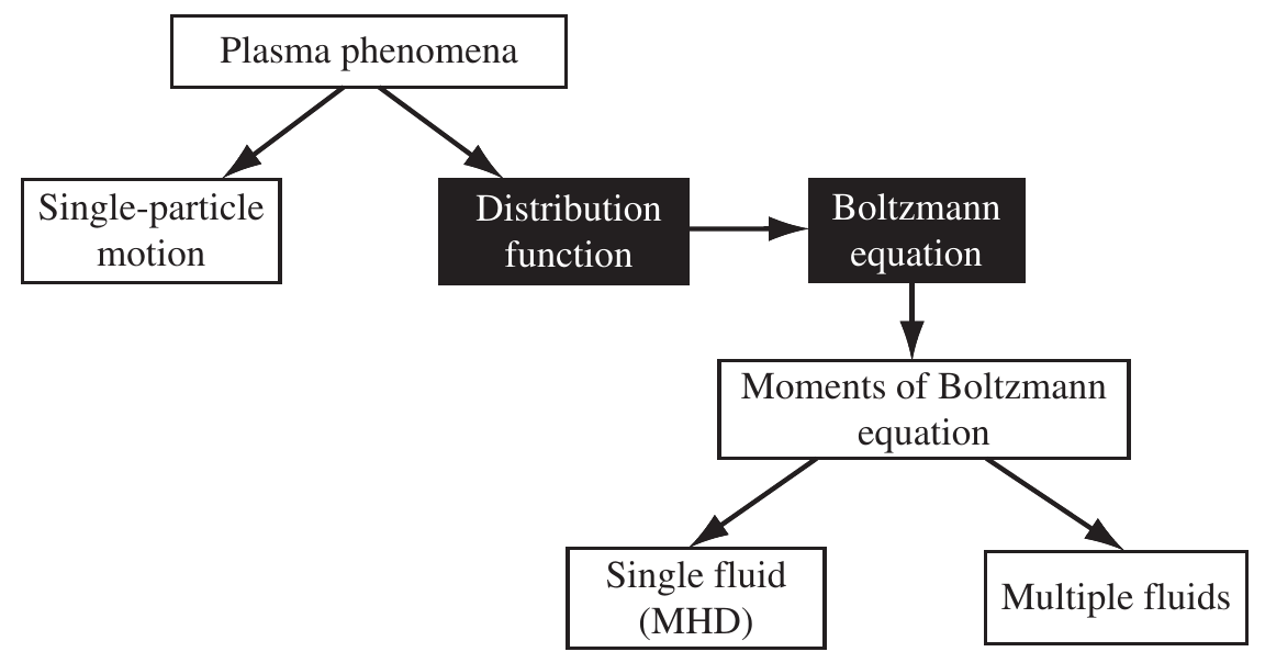
Hierarchy of plasma physics models

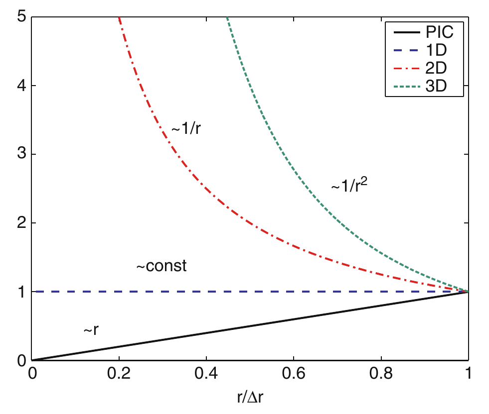
2.3 Validity of plasma models

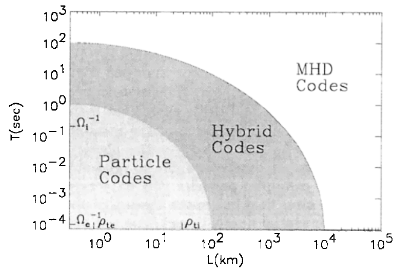
Range of validity of different plasma codes based on typical magnetospheric parameters: \(n=50cm^{-3}\), \(B=50 nT\), \(T_e=T_i=100 eV\) (Winske and Omidi 1996).

2.4 Validity of plasma models

Validity range of different plasma codes for a weakly collisional plasma [Credits: space.aalto.fi.]

2.5 Single-fluid MHD equations

Simplified single-fluid MHD equations (w/o explicit energy eq.)

\[ \nabla\cdot\vec{B}=0 \\ \nabla\times\vec{E}=-\frac{\partial \vec{B}}{\partial t} \\ \nabla\times\vec{B}=\mu_0\vec{J} \\ \vec{E}+\vec{V}\times\vec{B}= \eta \vec{J}\\ \]

\[ \frac{\partial \rho}{\partial t} + \nabla(\rho\vec{V})=0 \\ \rho\frac{d\vec{V}}{dt} = \vec{J}\times\vec{B}-\nabla P\\ P=K\rho^{5/3} \]

2.6 Fully-kinetic/Vlasov description

Fully-kinetic equations

\[ \nabla\cdot\vec{E}=\frac{\rho}{\epsilon_0}\\ \nabla\cdot\vec{B}=0\\ \nabla\times\vec{E}=-\frac{\partial \vec{B}}{\partial t}\\ \nabla\times\vec{B}=\mu_0\vec{J}+\mu_0\epsilon_0\frac{\partial \vec{E}}{\partial t}\\ \]

\[ \left[\frac{\partial}{\partial t} + \vec{v}\cdot\frac{\partial}{\partial \vec{x}}+\frac{q_{\alpha}}{m_{\alpha}}\left(\vec{E}+\vec{v}\times\vec{B}\right)\cdot\frac{\partial}{\partial \vec{v}}\right]f_{\alpha}=0\\ \rho=\sum\limits_{\alpha} q_{\alpha}\int\limits dv^3\,f_{\alpha}\\ \vec{J}=\sum\limits_{\alpha} q_{\alpha}\int dv^3\,\vec{v}f_{\alpha} \]

2.7 Advantages and drawbacks of plasma simulations codes

2.8 Your turn

1. How would you characterize the relation between astronomical observations, theory, and simulations?
2. Which example equations would use to describe the plasma and solve them in simulations?

3 Hands-on

3.1 Testing the computer setup

1. Login to local computers using your student accounts
2. Open command line
3. Run Jupyter Notebook/Lab: $ jupyter lab
4. Load basic Python libraries Numpy and Matplotlib
5. Plot an arbitrary analytical function (e.g., parabola, sin, cos,…)

If Jupyter Lab does not exist, run:

$ pip3 install --upgrade pip
$ pip3 install --user jupyterlab numpy scipy matplotlib
$ export PATH=$HOME/.local/bin:$PATH
$ jupyter lab

OR

• Instead of (1.–2.) Install and run Jupyter Lab on your computer.

4 Bibiography and references

4.1 Bibliography

• Büchner (2023)
• Büchner, Dum, and Scholer (2003)
• Matsumoto and Omura (1993)
• Jardin (2010)
• Winske and Omidi (1996)
• Lapenta (2012)
• Umeda (2012)
• Benáček et al. (2021)

5 Introduction to numerical methods

5.3 Modeling study

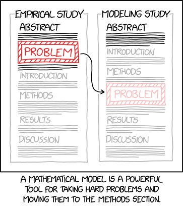
https://xkcd.com/2323/

6 ODEs

6.1 Introduction

• We want to solve the ordinary differential equation (ODE): \[ \frac{dy}{dt}=f(t,y), \] with the initial conditions \(y(t_0)=y_0\).

  \(\Rightarrow\) to find the value of \(y\) at a given \(t_n\): \(y_n:=y(t_n)\) (discretization).

• Idea

  1. To divide the interval \([t_0,t_N]\) in \(N\) intervals (\(N+1\) points), such as \(\Delta t=(t_N-t_0)/N\) and \(t_i=i\Delta t\) (\(n=0,1,2,\cdots,N\))
  2. To find a recursive expression relating \(y_n\) with \(\{y_{n-1},y_{n-2},\cdots\}\)

6.2 General form of an ODE

• Any ODE of order \(N\) can be written as a system of \(N\) first-order ODEs

\[ \frac{dy^{(1)}}{dt}=f^{(1)}\left(t,\{y^{(i)}\} \right)\\ \frac{dy^{(2)}}{dt}=f^{(2)}\left(t,\{y^{(i)}\}\right)\\ \cdots \qquad \cdots \\ \frac{dy^{(N)}}{dt}=f^{(N)}\left(t,\{y^{(i)}\}\right)\\ \]

\[ \] \[ \Leftrightarrow \]

\[ \qquad\frac{d\vec{y}}{dt}=\vec{f}(t,\vec{y})\qquad\qquad\qquad \nonumber\\\ \vec{y}=\begin{pmatrix} y^{(1)} \\ y^{(2)}\\\vdots \\ y^{(N)} \end{pmatrix},\qquad \vec{f}=\begin{pmatrix} f^{(1)}(t,\vec{y})\\ f^{(2)}(t,\vec{y})\\ \vdots \\ f^{(N)}(t,\vec{y}) \end{pmatrix} \qquad(1)\]

• Note that the RHSs do not have explicit derivatives.

6.3 Example

• Newton’s second law is a 2nd-order ODE that can be written as: \[ \frac{d^2x}{dt^2}=\frac{1}{m}F\left(t,\frac{dx}{dt},x\right) \]
• Let \[ y^{(1)} \equiv x, \quad y^{(2)} \equiv \frac{dx}{dt}=\frac{dy^{(1)}}{dt}. \] Then we have a system of two first-order ODEs in the form given by Equation 1: \[ \vec{y} \equiv \begin{pmatrix} x \\ \frac{dx}{dt} \end{pmatrix},\qquad \vec{f} \equiv \begin{pmatrix} y^{(2)}(t) \\ \frac{1}{m}F\left(t,y^{(1)},y^{(2)} \right) \end{pmatrix} \]

6.5 Euler’s method

• Simplest method to solve Equation 1: forward finite difference centered at \((t_i,y_i)\)

  (extrapolating the initial slope).

Euler’s method/Forward difference

\[ y_{i+1}=y_i + \Delta t f(t_i,y_i)+\mathcal{O}(\Delta t) \]

• The accuracy of this method is very low.
• More precise methods are necessary

Explicit methods

They give \(y_{i+1}\) in terms of already known values of \(y_i\) — e.g., the Euler method.

Implicit methods

They require to solve (invert) another equation (matrix) to obtain \(y_{i+1}\).

6.6 Accuracy and precision

6.7 Improved Euler’s method

• We can improve the naive Euler’s method by averaging the slopes at \((t_i,y_i)\) and \((t_{i+1},y_{i+1})\): \[ y_{i+1}^*=y_i+\Delta t\, f(t_i,y_i) \\ y_{i+1} =y_i+\Delta t\frac{f(t_i,y_i)+f(t_{i+1},y_{i+1}^*)}{2}\\ \]

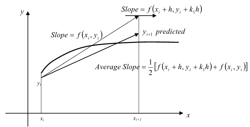
• This method predicts \(y_{i+1}\) by the direct Euler’s method and then corrects it.
• Basis for the predictor-corrector schemes.

6.8 Taylor expansion and finite differences

All finite difference expressions are based on

Taylor expansion

\[ f_{i+1}=f(x_i + \Delta x)=f_i + \Delta x f'(x_i) + \frac{\Delta x^2}{2!}f''(x_i) + \frac{\Delta x^3} {3!}f'''(x_i)+\cdots \]

Better accuracy can be obtained by considering more points \[ f_{i+1}-f_{i-1}= 2\Delta xf' + \frac{\Delta x^3}{3}f'''+\cdots \]

Central differences or 3 points formula

\[ f'(x_i)=\frac{1}{2\Delta x}\left[f_{i+1}-f_{i-1}\right]+\mathcal{O}(\Delta x^2) \]

And similarly, using \(f_{i+2}-f_{i-2}\),

5 points formula

\[ f'(x_i)=\frac{1}{12\Delta x}\left[f_{i-2}-8f_{i-1}+8f_{i+1}-f_{i+2}\right]+\mathcal{O}(\Delta x^4) \]

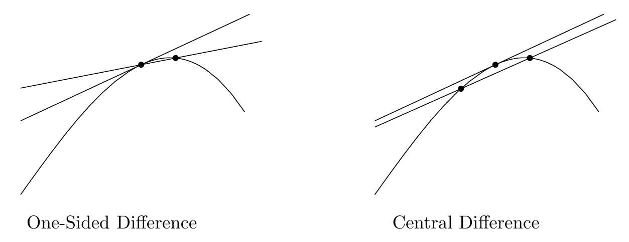
6.9 Finites difference: forward vs centered

6.10 Second order derivatives with finite differences

By using (only) \(f_{i+1}\) and \(f_{i-1}\), we can get ,

Second order derivatives

\[ f''(x_i)=\frac{f_{i+1} - 2f_i + f_{i-1}}{\Delta x^2}+\mathcal{O}(\Delta x^2) \qquad(2)\]

We can also get this by using 1st-order central differences \[ f''(x_i)=\frac{d}{dx}\left(\frac{df}{dx}\right)=\lim_{\Delta x\to 0}\frac{f'_{i+1/2}-f'_{i-1/2}}{\Delta x}\approx \frac{(f_{i+1}-f_i)/\Delta x-(f_{i}-f_{i-1})/\Delta x}{\Delta x} \]

It is possible to systematically obtain higher order derivatives with arbitrary accuracy. See a list in http://en.wikipedia.org/wiki/Finite_difference_coefficients

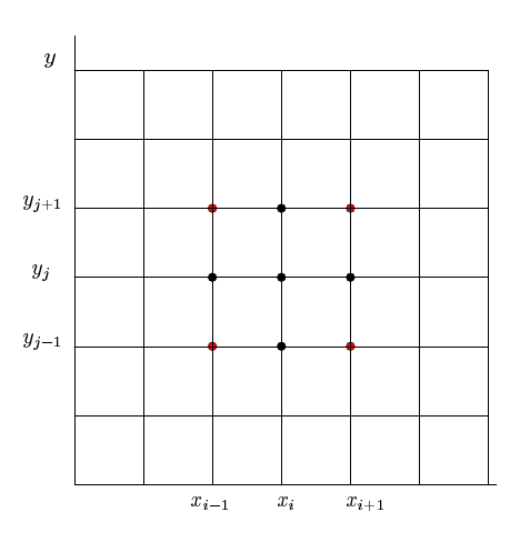
6.11 Finite differences in two variables

For 2D domains (e.g., in PDEs), we can generalize the previous procedure by using, e.g, a five-point stencil \[ \left(\frac{\partial^2 f}{\partial x \partial y}\right)_{i,j}=\frac{\left(\frac{\partial f}{\partial y}\right)_{i+1,j}-\left(\frac{\partial f}{\partial y}\right)_{i-1,j}}{2\Delta x} \approx \frac{f_{i+1,j+1}-f_{i+1,j-1}-f_{i-1,j+1}+f_{i-1,j-1}}{4\Delta x\Delta y} \]

6.12 Your turn:

Task 1

1. Select a differential method and numerically solve the differential equation \[ \frac{dx}{dt} = f(t) = cos(t) \qquad(3)\] with \(\Delta t = 0.01\), and initial condition x(t=0) = 0, and interval \(t = [0,6\)\(]\).

2. Compare various methods with analytical solution of Equation 3

3. Analyze impact of the time step \(\Delta t\) on the quality of the solution

4. How much differs run-time between various time steps?

   Tip: For timing the computation use “%%timeit” command at the beginning of the notebook cells.

Task 2

Analytically prove Equation 2, using the formula for the first derivative

7 PDEs

7.1 Characteristics of PDEs

• Curves in the space of independent variables of a PDE, along which the PDE has only total differentials.

  By integrating along those curves one can find the solutions of such a PDE.

• Example: \[ a\frac{\partial u}{\partial t} + b\frac{\partial u}{\partial x} = c \] with solutions \(u=u(x(t),t)\).

• Total derivative of \(u\): \[ \frac{du}{dt}=\frac{\partial u}{\partial x}\frac{dx}{dt} + \frac{\partial u}{\partial t} \]

• The characteristics are the solutions of: \[ \frac{dx}{dt}=\frac{b}{a},\;\; \frac{du}{dt}=\frac{c}{a} \] which means, for \(u(x_0,0)=u_0\), \[ x = x_0 + \frac{b}{a}t\\ u = u_0 + \frac{c}{a}t\\ \]

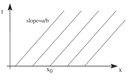
7.2 Characteristics of PDEs

• Curves in the space of independent variables of a PDE, along which the PDE has only total differentials
• Solution/characteristics: \[ x = x_0 + \frac{b}{a}t\\ u = u_0 + \frac{c}{a}t\\ \]
• Note that if \(c=0\), \(u\) is constant on the characteristics.
• For non constant \(c\), \(u\) grows linearly in time along a characteristic \(\Rightarrow\) the initial profile \(u(x,0)\) already determines the solution along the characteristics

7.3 Characteristics of PDEs

• For the second order PDE: \[ A\frac{\partial^2 f}{\partial x^2} + B\frac{\partial^2 f}{\partial x \partial y} + C\frac{\partial^2 f}{\partial y^2} + G = 0 \]

The characteristics are the solutions of: \[ \frac{dy}{dx} = \frac{B}{2A}\pm \frac{1}{2A}\sqrt{B^2 - 4AC} \]

This equation is:

• elliptic: \(B^2 - 4AC < 0\). No real solutions.
• parabolic if \(B^2 - 4AC = 0\). One real solutions.
• hyperbolic if \(B^2 - 4AC > 0\). Two real solutions.

7.4 Systems \(n\) of 1st order PDEs

• It is possible to write such a system of \(n\) PDEs in two dependent variables \(x\) and \(y\) as: \[ \left(\bar{A}^T\frac{dy}{dx} - \bar{B}^T \right)\cdot \vec{L} = 0 \] where \(\vec{L}\) is a vector of dimension \(n\), \(\bar{A}^T\), \(\bar{B}^T\), are \(n\times n\) matrices. The determinant leads to a \(n\)th order equation for \(dy/dx\), which can be classified as:
  • elliptic for no real roots
  • parabolic for \(1\) to \(n-1\) real roots and no complex roots
  • hyperbolic for \(n\) real roots

7.5 Classification

7.6 Linear Second Order PDEs in 2 independent variables

• The most general form of a linear second order PDE with independent variables \(x,y\) and dependent variable \(f(x,y)\) is: \[ A\frac{\partial^2 f}{\partial x^2} + B\frac{\partial^2 f}{\partial x \partial y} + C\frac{\partial^2 f}{\partial y^2} + D\frac{\partial f}{\partial x} + E\frac{\partial f}{\partial y} + G = 0 \]

  \(A,\dots, G\) are constants.

This equation is:

• elliptic if \(B^2 - 4AC < 0\)

• parabolic if \(B^2 - 4AC = 0\)

• hyperbolic if \(B^2 - 4AC > 0\)

7.7 Linear Second Order PDEs in 2 independent variables

• Elliptic (\(B^2 - 4AC < 0\)): Steady state problems (gravity, electrostatic). Laplace equation (2D): \[ \nabla ^2\phi = \frac{\partial^2 \phi}{\partial x^2} + \frac{\partial^2 \phi}{\partial y^2} =0 \]
• Parabolic (\(B^2 - 4AC = 0\)): Time-dependent fluid equations where conduction/diffusion are important. Heat conduction equation \[ \frac{\partial T}{\partial t}=k\frac{\partial^2 T}{\partial x^2} \]
• Hyperbolic ( \(B^2 - 4AC > 0\)): Time-dependent fluid eqs where convection is important. Vibration, propagation. Wave equation \[ \frac{\partial^2U}{\partial t^2}=c^2\frac{\partial^2 U}{\partial x^2} \]

7.8 Multiple independent variables

• Let us consider a single dependent variable \(f\) but \(m\) independent variables: \[ \sum_{j=1}^{m} \sum_{k=1}^{m} a_{jk} \frac{\partial^2 f}{\partial x_j \partial x_k} + H=0 \] The character of this eq is determined by the eigenvalues (EV) of the matrix \(A=(a_{jk})\).
• This equation is
  • elliptic if all the EVs \(\neq0\) and all the same sign.
  • parabolic if any EV is 0
  • hyperbolic if all the EVs \(\neq0\) and all but one have the same sign.

7.9 Hyperbolic PDEs

• Example: wave equation: \[ \frac{\partial^2 u}{\partial t^2} - c^2\frac{\partial^2 u}{\partial x^2} = 0 \qquad(4)\]
• Solution: Two sine waves, traveling into the positive \((+x)\) and negative \((-x)\) directions.
• Typical property: propagation of information through a system via waves (e.g. sound waves) along the characteristics of the equation.
• Examples: various time dependent forms of fluid equations without dissipation: heat conduction, viscosity, resistivity
• The number of initial conditions (this case: dependent variables and their derivatives) has to correspond with the number of unknowns or waves.
• Any point source along \(x\) will influence its vicinity along the corresponding characteristics (two straight lines for Eq. Equation 4.

7.10 Hyperbolic PDEs

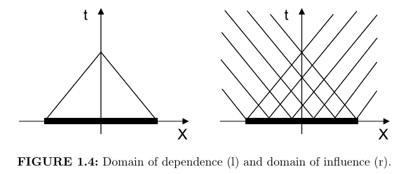
Characteristics of a hyperbolic wave equation. Left: Domain of dependence. Right: Domain of influence Jardin (2010)

7.11 Parabolic PDEs

• Example: heat conduction, magnetic flux diffusion, evolution of a velocity distribution function in velocity space due to particle collisions. \[ \frac{\partial u}{\partial t}= \sigma \frac{\partial^2 u}{\partial x^2} \qquad(5)\]
• Solution for one initial condition (typically Dirichlet) and two boundary conditions: \[ u(x,t) = \sin(\pi x)\exp(-\pi^2 t) \]
• Only one characteristic
• Any local perturbation influences the entire domain, but with decreasing magnitude for increasing distance from the source of the perturbation.

7.12 Elliptic PDEs

• Typical for steady state problems (time-independent limit of hyperbolic or parabolic eqs), or for potentials (Poisson’s equation).
• Example: 2D Poisson equation (Or Laplace’s equation if the RHS=0) \[ \frac{\partial^2 u}{\partial x^2} + \frac{\partial^2 u}{\partial y^2} = \rho(x,y) \qquad(6)\]
• Solution for 4 boundary conditions: \[ u(x,y) = \sin(\pi x)\exp(-\pi y) \]
• No real characteristics
• Both the maximum and minimum are assumed on the boundary \(\partial R\).
• Any disturbance on the interior influences the entire computational domain.

7.13 Flux-Conservative Initial Value Problems

• A large-class of initial value PDEs in 1D can be cast into the form of a flux-conservative equation: \[ \frac{\partial \vec{u}}{\partial t} = -\frac{\partial \vec{F}(\vec{u}, \frac{\partial \vec{u}}{\partial \vec{x}})}{\partial x} \] where \(\vec{F}\) is the conserved flux
• For example, the 1D wave equation can be written as: \[ \frac{\partial r}{\partial t} = c\frac{\partial s}{\partial x}\\ \frac{\partial s}{\partial t} = c\frac{\partial r}{\partial x}\\ \] where \(r=c \frac{\partial u}{\partial x}\) and \(s= \frac{\partial u}{\partial t}\). Then, the flux is given by the linear matrix relation: \[ \vec{F}(\vec{u}) = \begin{pmatrix} 0&-c\\ -c&0\\ \end{pmatrix} \cdot \vec{u} \]

7.14 Boundary conditions

Let us define a domain, its boundary \(\partial R\), the coordinates \(n\) (outward normal to the boundary) and \(s\) (along the boundary), and the functions \(f\) and \(g\) on the boundary. The three types of BCs are:

1. Dirichlet conditions: \(u=f\) on \(\partial R\)
2. Neumann conditions: \(\frac{\partial u}{\partial n} =f\) or \(\frac{\partial u}{\partial s} =g\) on \(\partial R\)
3. Mixed (Robin) conditions: \(\frac{\partial u}{\partial n} + ku=f, \;\; k>0\) on \(\partial R\).

7.15 Initial vs Boundary conditions

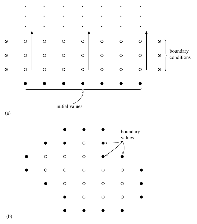
(a) Initial (Cauchy) vs (b) Boundary value problems (Press et al. (2007)). In (a) the arrows indicate time.

7.16 Stability

7.17 Von Neumann stability analysis

• Based on a finite Fourier transform to convert spatial differences into an expression with the \(\xi\), such as the independent solutions (eigenmodes) are: \[ u_j^n=\xi^n(k) e^{ikj\Delta x} \qquad(7)\] \(j\) is the space index, \(n\) is the time index, \(i\) the imaginary unit, \(k\) the wavenumber, \(\Delta x\) the grid cell spacing.
• The difference equation will be unstable if \(|\xi(k)|>1\) for some \(k\). This means exponential growing modes.
• von Neumann analysis is local.

7.18 Von Neumann stability analysis 2

• Example: numerically unstable hyperbolic equation: wave equation written as a system of 1st order eqs (each one is sometimes called “advective equations”). \[ \frac{\partial u}{\partial t} = -v \frac{\partial u}{\partial x} \] The (forward time centered space) FTCS representation is: \[ \frac{u_j^{n+1} - u_j^{n}}{\Delta t} = -v \left(\frac{u_{j+1}^{n} - u_{j-1}^{n}}{2\Delta x} \right) \qquad(8)\]
• Replacing Equation 7 in Equation 8 we get: \[ \xi(k)=1-i\frac{v\Delta t}{\Delta x}\sin(k\Delta x) \] which is \(>1\) for all \(k\), so that the scheme is unstable.

7.19 Von Neumann stability analysis 3

• Example: numerically stable hyperbolic equation: let us replace the time derivative in Equation 8 by its average: \[ u_j^{n+1} = \frac{1}{2}\left(u_{j+1}^{n} + u_{j-1}^{n}\right) -\frac{v\Delta t}{2\Delta x} \left(u_{j+1}^{n} - u_{j-1}^{n} \right) \qquad(9)\] (this is known as the Lax method), which gives the amplification factor: \[ \xi(k)=\cos(k\Delta x)-i\frac{v\Delta t}{\Delta x}\sin(k\Delta x) \] and it leads to the stability condition:

Courant-Friedrichs-Lewy

Courant-Friedrichs-Lewy stability condition (CFL, Courant condition): \[ \frac{v\Delta t}{\Delta x}\leq 1 \] Example: 2nd order hyperbolic wave equation (derived from the determinant of a matrix).

7.20 CFL condition

CFL condition Jardin (2010)

7.21 Von Neumann stability analysis 4

• It can be proven that Equation 9 is equivalent to a FTCS (forward time-centered space) representation of \[ \frac{\partial u}{\partial t} = -v \frac{\partial u}{\partial x} + \frac{(\Delta x)^2}{2\Delta t}\nabla^2 u \] where the extra term is a diffusion/dissipative term. Then, the Lax scheme is said to have numerical dissipation or viscosity.

7.22 Methods

7.23 Solution methods for parabolic equations 1

• Diffusion equation in 1D \[ \frac{\partial u}{\partial t}= D \frac{\partial^2 u }{\partial x^2} \qquad(10)\] where \(D\) is the diffuction parameter.

  This can also be written as a flux-conservative equation, with F=-\(D \frac{\partial u}{\partial x}\).

• \(D\geq 1\) in order for Eq. Equation 10 to be stable.

• Applying a FTCS scheme we get: \[ \frac{u_j^{n+1} - u_j^{n}}{\Delta t} = D \left(\frac{u_{j+1}^{n} -2u_j^n + u_{j-1}^{n}}{(\Delta x)^2} \right) \qquad(11)\]

7.24 Solution methods for parabolic equations 2

• The amplification factor is: \[ \xi(k)=1 -\frac{4D \Delta t}{(\Delta x)^2}\sin(k\Delta x/2) \] leading to the stability criterion: \[ \frac{2D\Delta t}{\Delta x}\leq 1 \qquad(12)\] the maximum allowed timestep is approx. the diffusion time across a cell of width \(\Delta x\).
• In general, the diffusion time across a spatial scale of size \(\lambda\) is \(\tau\sim \frac{\lambda^2}{D}\), which leads to a number of timesteps (based on Equation 12) of order \(\frac{\lambda^2}{\Delta x^2}\) \(\rightarrow\) too many.

7.25 Solution methods for parabolic equations 3

• One solution to change the small CFL timestep of the diffusion eq. is the Crank-Nicholson scheme, second-order accurate in time.
• Average of explicit and implicit FTCS schemes: \[ \frac{u_j^{n+1} - u_j^{n}}{\Delta t} = \frac{D}{2}\left(\frac{(u_{j+1}^{n+1} -2u_j^{n+1} + u_{j-1}^{n+1}) +(u_{j+1}^{n} -2u_j^{n} + u_{j-1}^{n}) }{(\Delta x)^2} \right) \qquad(13)\]
• The amplification factor predicts that the method is stable for any \(\Delta t\)
• Crank-Nicholson also works well for Schrödinger-like eqs. \[ i\frac{\partial \psi}{\partial t} = -\frac{\partial ^2\psi}{\partial x^2} + V(x)\psi \]

7.26 Solution methods for elliptic PDEs

• 2D Poisson equation \[ \frac{\partial^2 u}{\partial x^2} + \frac{\partial^2 u}{\partial y^2} = R(x,y) \qquad(14)\] with Dirichlet boundary conditions: \[ u(0,y), u(L,y) \qquad 0<y<L \] and \[ u(x,0), u(x,L) \qquad 0<x<L \]

The 2nd order finite difference equation for \(j,k\)-element (derived by the Taylor expansion) is: \[ u_{j+1,k} + u_{j-1,k} + u_{j,k+1} + u_{j,k-1} - 4u_{j,k} = \Delta x^2 R_{j,k}. \qquad(15)\] Let the \((N+1)^2\) vector of unknowns be denoted by \(\vec{x}\), which contains \(u_{j,k}\) elements.

The matrix form of Equation 15 is \(\hat{A}\cdot\vec{X}=\vec{b}\)

7.27 Solution methods for elliptic PDEs

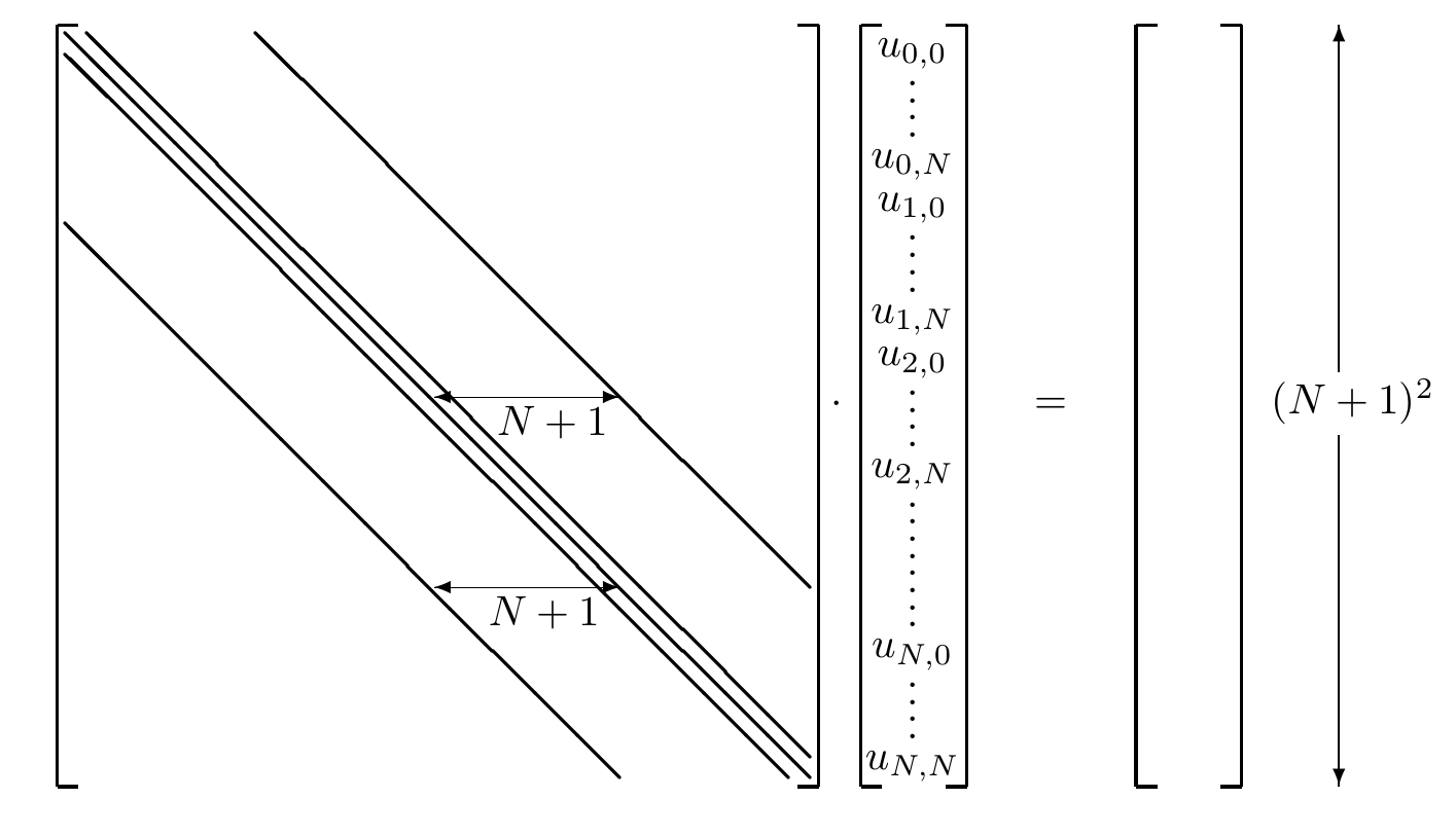
Sparse matrix \(\hat{A}\):

• Must be inverted to solve for the unknowns (although the actual inverse is not normally calculated). Some methods are:
  • Direct inversion using Gauss or LU decomposition
  • Direct inversion using block tri-diagonal methods
  • Iterative methods (multigrid, Krylov space methods). A physical approach involves adding time derivatives terms (converting it to parabolic/hyperbolic equations), and advancing it in time until a steady state is obtained.
  • Direct methods based on transform techniques (e.g., Fourier transformation)

7.28 Multigrid methods

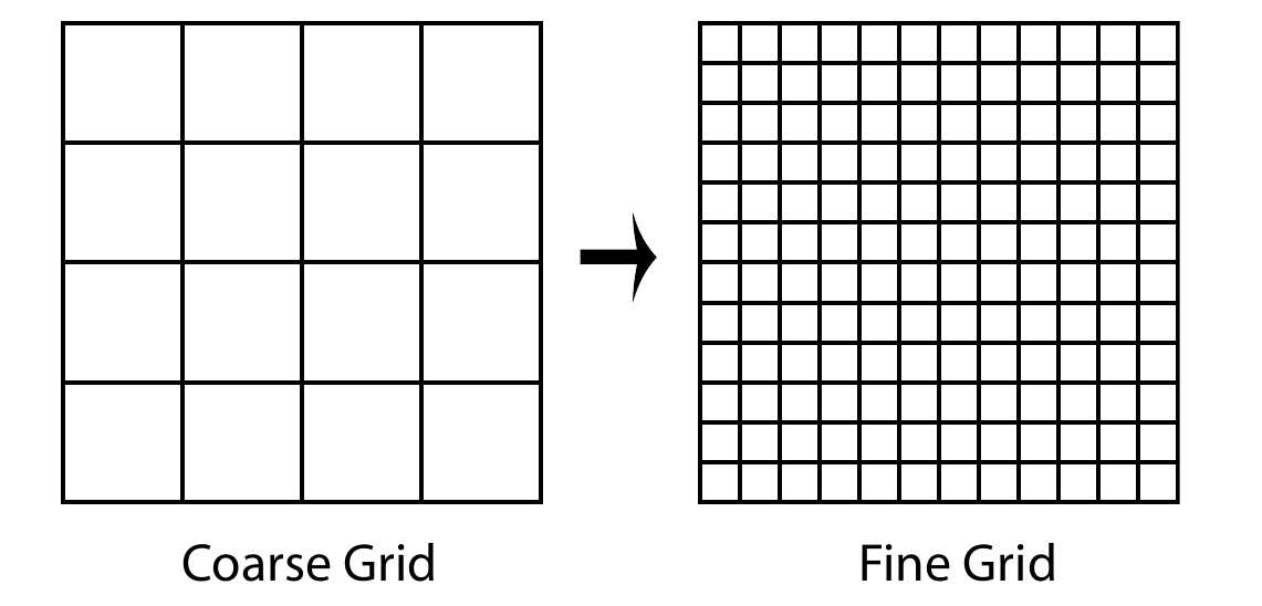
Schematics of multigrid method

• Iterative methods benefit greatly from a good initial guess: A coarse grid solution can be used to initialize a finer grid iteration
• On a given grid, the short wavelengths components of the error decay much faster than the long wavelengths. So, the coarse mesh is more efficient in handling long components of the error but the fine mesh is needed for the short wavelength components.
• The error satisfies the same matrix eqs. as the unknown.
• Two basic steps: nested iteration (for the initial guess), coarse grid correction.

7.29 Fast Fourier methods

• Fourier (spectral) methods can be applied to solve boundary problems (e.g., elliptic equations) that lead to large sparse linear systems of the form \(\hat{A}\cdot\vec{u}=\vec{b}\)
• The algorithm is based on a Fast Fourier transform (FFT), a clever trick to avoid the calculation of \(N^2\) multiplications and \(N(N-1)\) that are required for a direct finite Fourier transform. Instead, if \(N\) is equal to a power of 2, it leads to a product of \(log_2(N)\) sparse matrices.
• It works best when the PDE has constant coefficients and the boundaries coincide with the coordinate lines.

8 References

Benáček, Jan, Patricio A. Muñoz, Alina C. Manthei, and Jörg Büchner. 2021. “Radio Emission by Soliton Formation in Relativistically Hot Streaming Pulsar Pair Plasmas” 915 (2): 127. https://doi.org/10.3847/1538-4357/ac0338.

Boyd, T. J. M., and J. J. Sanderson. 2003. The Physics of Plasmas.

Büchner, Jörg. 2023. Space and Astrophysical Plasma Simulation. Methods, Algorithms, and Applications. https://doi.org/10.1007/978-3-031-11870-8.

Büchner, Jörg, C Dum, and M Scholer. 2003. Space Plasma Simulation. Berlin Heidelberg: Springer-Verlag.

Jardin, S. 2010. Computational Methods in Plasma Physics. CRC Press.

Lapenta, Giovanni. 2012. “Particle simulations of space weather.” J. Comput. Phys. 231 (3): 795–821. https://doi.org/10.1016/j.jcp.2011.03.035.

Matsumoto, H, and Y Omura. 1993. Computer Space Plasma Physics : Simulation Techniques and Software. Terra Scientific Publishing Company. https://www.terrapub.co.jp/e-library/cspp/.

Press, William H., Saul A. Teukolsky, William T. Vetterling, and Brian P. Flannery. 2007. Numerical Recipes: The Art of Scientific Computing. Third Edition. Cambridge University Press. https://doi.org/10.1137/1031025.

Umeda, Takayuki. 2012. “Simulation of Collisionless Plasma With the Vlasov Method.” In Int. Conf. Simul. Technol., edited by Brian S. Doherty and Amy N. Molloy, 315–32. Nova Science Publishers. http://www.jsst.jp/e/JSST2012/extended_abstract/pdf/12.pdf.

Winske, D., and N. Omidi. 1996. “A nonspecialist’s guide to kinetic simulations of space plasmas.” J. Geophys. Res. 101 (A8): 17287. https://doi.org/10.1029/96JA00982.