Lecture 7: Fluid and MHD – Lecture

Jan Benáček

Institute for Physics and Astronomy, University of Potsdam

November 30, 2023

Table of contents

• 1 Lecture overview
• 2 MHD physics
• 3 MHD equations
• 4 Discretization schemes for simple fluids PDEs
• 5 System of fluids/MHD equations

1 Lecture overview

Table of Contents 1/2

• 19.10. Introduction + numerical methods summary
• 26.10. Numerical methods for differential equations - lecture + hands-on
• 02.11. Test particle approach — lecture
• 09.11. Test particle approach — hands-on
• 16.11. PIC method — lecture
• 23.11. PIC method — hands-on
• 30.11. Fluid and MHD — lecture

Table of Contents 2/2

• 07.12. Fluid and MHD — hands-on
• 14.12. Radiative transfer — lecture
• 11.01. Radiative transfer — hands-on
• 18.01. HPC computing — lecture + hands-on
• 25.01. Advanced — Smooth particle hydrodynamics method — lecture
• 01.02. Advanced — Hybrid, Gyrokinetics — lecture
• 08.02. Advanced — Vlasov and Linear Vlasov dispersion solvers — lecture

2 MHD physics

2.1 Introduction

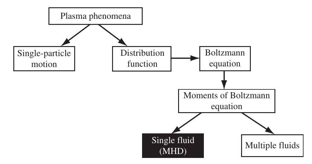
2.2 MHD plasma model

• Fluid description: it uses a few macroscopic quantities, averages of the distribution function (mean velocity, pressure/temperature). Valid for or near thermodynamic equilibrium.

2.3 Validity of the MHD model

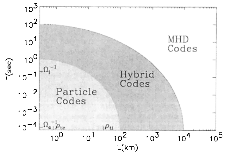
Range of validity of different plasma codes based on typical magnetospheric parameters: \(n=50cm^{-3}\), \(B=50 nT\), \(T_e=T_i=100 eV\) (Winske and Omidi (1996)).

2.4 Approximation and definitions in single-fluid MHD

• Plasma is charge-neutral because \(L \gg \lambda_{de}\) (Poisson eq. is superfluous)
• \(V\ll c\) (no displacement current in Ampere’s equation)
• \(T\gg\Omega_{ce},\Omega_{ci}\) (electron/ion cyclotron frequencies)
• \(L\gg d_e, d_i\) (electron/ion skin depths) and \(L\gg \rho_e, \rho_i\) (electron/ion gyroradius) \[ \vec{J} = \sum_{\alpha}q_{\alpha}n_{\alpha}\vec{V}_{\alpha}\\ \vec{V}=\frac{1}{\rho}\sum_{\alpha}m_{\alpha}n_{\alpha}\vec{V}_{\alpha} \\ \rho = \sum_{\alpha} m_{\alpha}n_{\alpha} \]

3 MHD equations

3.1 Magnetohydrodynamics

Title text of https://xkcd.com/1851/: “Magnetohydrodynamics combines the intuitive nature of Maxwell’s equations with the easy solvability of the Navier-Stokes equations. It’s so straightforward physicists add”relativistic” or “quantum” just to keep it from getting boring”.

3.2 Continuity equation

• Equation for the time evolution of \(\rho(\vec{x},t)\), unknown bulk flow velocity \(\vec{V}(\vec{x},t)\).
• Conservation of mass: variation of the mass in a volume \(V\) must be entirely due to the inflow or outflow of mass through their boundary \(\partial V\). \[ \frac{\partial }{\partial t}\int \rho dV = -\int_{\partial V} \rho\vec{V}\cdot\vec{n}dS \]
• Differential form: \[ \frac{\partial \rho}{\partial t} + \nabla\cdot(\rho \vec{V})=0 \]
• Approximation: for incompressible fluids (\(\nabla\cdot\vec{V}=0\)) it becomes the advection equation. \[ \frac{\partial \rho}{\partial t} +\vec{V}\cdot\nabla\rho=\frac{d\rho}{dt}=0 \]

3.3 Momentum equation

• Equation for the time evolution of \(\vec{V}(\vec{x},t)\), unknown: pressure tensor \(\bar{P}(\vec{x},t)\).
• Integral form: Total momentum in a volume is the volume integral of \(\rho\vec{V}\), but it is also necessary to consider the forces on the surface due to the plasma pressure surrounding the volume and the electromagnetic forces
• Differential form \[ \frac{\partial \rho \vec{V}}{\partial t} +\nabla\cdot(\rho \vec{V} \vec{V})= - \nabla\cdot\bar{P} + qn(\vec{E}+\vec{V}\times\vec{B}) \]
• Approximation: for a scalar pressure, gravity force instead of Lorentz force, one obtains the Euler’s equation (a simplified version of Navier-Stokes equation without viscosity). \[ \frac{\partial \vec{V}}{\partial t} + \vec{V}\cdot\nabla\vec{V} = -\frac{1}{\rho}\nabla\bar{P} +\vec{g}. \]

3.4 Approximation: Burgers’ equation

• Neglecting pressure and external force terms, and assuming a simple (kinematic) viscosity (\(\nu=\eta/\rho\), also called diffusion coefficient), we get the Burgers’ equation \[ \frac{\partial \vec{V}}{\partial t} + \vec{V}\cdot\nabla\vec{V} -\nu \nabla^2\vec{V}= 0 \]
• In the inviscid limit \(\nu=0\), it becomes a 1st order hyperbolic PDE (advective type), prototype for shock wave equations: conservation equations that can develop steep discontinuities: \[ \frac{\partial \vec{V}}{\partial t} + \vec{V}\cdot\nabla\vec{V} = 0 \]

3.5 Energy equation

• Equation for the time evolution of \(\bar{P}(\vec{x},t)\), unknown: heat flux \(\bar{L}(\vec{x},t)\), related to the third momenta of the distribution function. \[ \frac{1}{\gamma - 1}\left( \frac{\partial \bar{P}}{\partial t} + \nabla\cdot(\bar{P}\vec{V}) \right) = -(\bar{P}\cdot\nabla)\cdot\vec{V} - \nabla\cdot\vec{L} \] where \(\gamma\) is the ratio of specific heats, \(\gamma=5/3\) for an ideal gas with 3 degrees of freedom. Other possible choices are \(\gamma=1\) for isothermal systems, or \(\gamma=\infty\) for incompressible systems.
• The pressure tensor \(\bar{P}\) is usually simplified as a scalar pressure \(p\).

3.6 Approximation: heat conduction

• Using an ideal gas law \(p=nk_BT\), scalar pressure, constant density, heat flux driven by a temperature gradient: \(\vec{L}=-\kappa\nabla T\), we get the diffusion/heat conduction equation: \[ \frac{\partial T}{\partial t} = \mu\nabla^2 T. \]

3.7 Equation of state

• The equation for moment of order \(n\) always requires the one for the moment of order \(n+1\) (i.e: an unknown in the continuity eq is the velocity \(\vec{V}\), whose evolution is calculated by the momentum equation).
• One way to close this infinite number of equations is by truncating at some point: usually by means of a thermodynamic (EOS).
• An EOS usually relates pressure \(p\) and density \(n\).

3.8 Equation of state

Equations of state

• Isothermal: \(p=nk_BT\), or \(\nabla p=nk_B\nabla T\) (slow time variations, plasma exchanges energy with its surroundings). Energy equation required, heat flux assumed to be: \(\vec{L}=-\kappa \nabla T\).
• Adiabatic: \(pn^{\gamma} =C\) or \(\nabla p/p=\gamma \nabla n/n\) (fast time variations, plasma does not exchange energy with its surroundings, no heat flow). Typically \(\gamma=1+2/N_d\) (\(N_d\): degrees of freedom), ratio of specific heats.

3.9 Ohm’s law

• Assumption: \(\vec{J} = \sigma \vec{E}\) or $ = $ (typical Ohm’s law in circuit theory \(V=IR\))
• In the non-relativistic approximation, the electric field in the frame of reference of a fluid element moving with velocity \(\vec{V}\) is \(\vec{E} + \vec{V}\times\vec{B}\) (Galilean transformation). Theen, the Ohm’s law is: \[ \vec{E} + \vec{V}\times\vec{B} = \eta\vec{J} \]

3.10 Single-fluid MHD

Simplified single-fluid MHD equations (w/o explicit energy eq.)

\[ \nabla\cdot\vec{B}=0\\ \nabla\times\vec{E}=-\frac{\partial \vec{B}}{\partial t}\\ \nabla\times\vec{B}=\mu_0\vec{J} \\ \vec{E}+\vec{V}\times\vec{B}= \eta \vec{J} \]

\[ \frac{\partial \rho}{\partial t} + \nabla(\rho\vec{V})=0 \\ \rho\frac{d\vec{V}}{dt} = \vec{J}\times\vec{B}-\nabla P\\ P=K\rho^{5/3} \]

3.11 Induction equation

Using Faraday’s, Ampere’s and the Ohm’s law, we obtain

Induction equation

\[ \frac{\partial\vec{B}}{\partial t}=\underbrace{\nabla\times\left(\vec{V}\times\vec{B}\right)}_{convection} +\underbrace{\frac{\eta}{\mu_0}\nabla^2\vec{B}}_{\rm diffusion} \]

Taking the ratio between the two terms, we obtain the Magnetic Reynolds number \[ R_M=\frac{{\rm convection}}{{\rm diffusion}}=\mu_0 V L/\eta \]

• \(R_m \gg 1\): Convection/flow dominates
• \(R_m \ll 1\): Diffusion dominates.

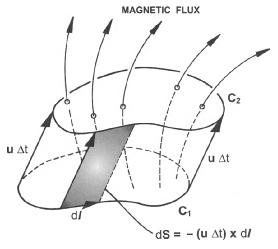
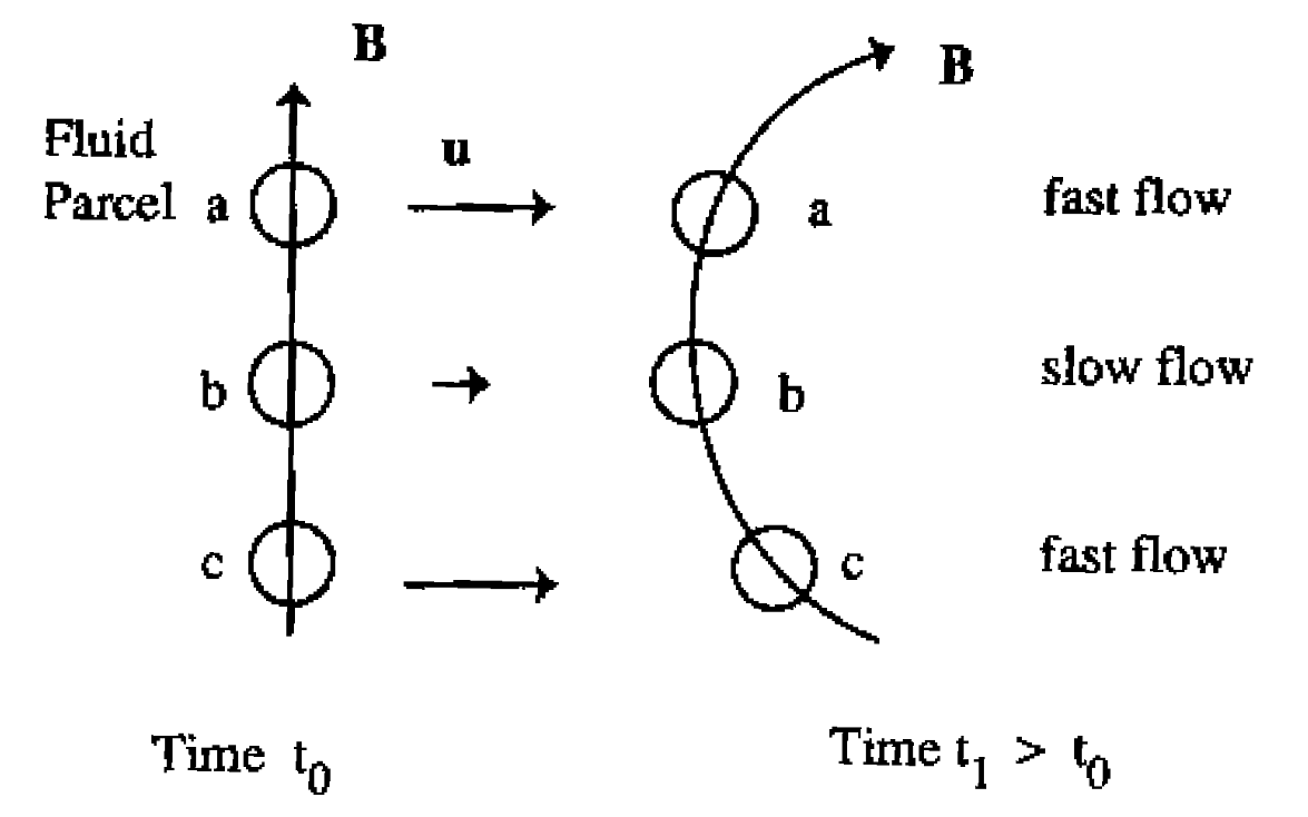
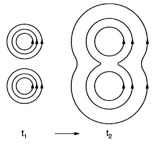
3.12 Frozen-in magnetic flux: The Alfvén theorem

• If convection dominates (diffusion negligible), \(R_m\gg 1\)

\[ \frac{\partial\vec{B}}{\partial t}=\nabla\times\left(\vec{V}\times\vec{B}\right) \;\;\text{or}\;\; \vec{E}+\vec{V}\times\vec{B}=0 \]

Alfvén’s theorem

\[ \frac{D\Phi}{Dt}=0 \;\;\text{or}\;\; \Phi=\int\vec{B}\cdot d\vec{S}=\text{constant} \]

3.13 Magnetic diffusion

• If diffusion dominates \(R_m\ll 1\) \[ \frac{\partial\vec{B}}{\partial t}=\frac{\eta}{\mu_0}\nabla^2\vec{B} \] A simple solution of the diffusion equation is \[ B = B_0{\rm exp}\left(\pm t/\tau_d\right), \qquad \mathrm{with} \qquad \tau_d=\mu L_B^2/\eta. \]

Magnetic diffusion (Baumjohann and Treumann (1997)).

3.14 Single-fluid MHD

Evolution MHD equations

\[ \frac{\partial\vec{B}}{\partial t}=\nabla\times\left(\vec{V}\times\vec{B}\right) +\frac{\eta}{\mu_0}\nabla^2\vec{B}\\ \frac{\partial \rho}{\partial t} =- \nabla(\rho\vec{V})=0 \\ \rho\frac{d\vec{V}}{dt} =\frac{1}{\mu_0}(\nabla\times\vec{B})\times \vec{B}-\nabla P \]

4 Discretization schemes for simple fluids PDEs

4.1 Methods for diffusion equations

4.2 Methods for diffusion equations

• 1D diffusion (parabolic) equation is \[ \frac{\partial f}{\partial t} - \alpha \frac{\partial^2 f}{\partial x^2} =0 \]

• This equation can be arranged as a flux-conservative equation: \[ \frac{\partial f}{\partial t} = -\frac{\partial F(f, \frac{\partial f}{\partial x})}{\partial x} \quad \mathrm{with} \quad F=-\alpha \frac{\partial f}{\partial x}. \]

• Examples

  • Heat conduction equation (from energy equation)
  • Magnetic diffusion (from induction equation)

4.3 Methods for diffusion equations: FTCS

• The forward time centered space (FTCS) difference scheme is: \[ f_j^{n+1} = f_j^n + s\Delta x^2 L_{xx} f_j^n \] where \(s:=\alpha\Delta t/\Delta x^2\) and the discretized (centered in space) Laplacian operator is: \[ L_{xx} f_j^n=\frac{1}{\Delta x^2}(f_{j-1}^n - 2f_{j}^n + f_{j+1}^n ) \] This means: \[ \frac{f_j^{n+1} - f_j^{n}}{\Delta t} = \alpha \left(\frac{u_{j+1}^{n} -2f_j^n + f_{j-1}^{n}}{(\Delta x)^2} \right). \qquad(1)\]

4.4 Forward time centered space (FTCS) difference scheme

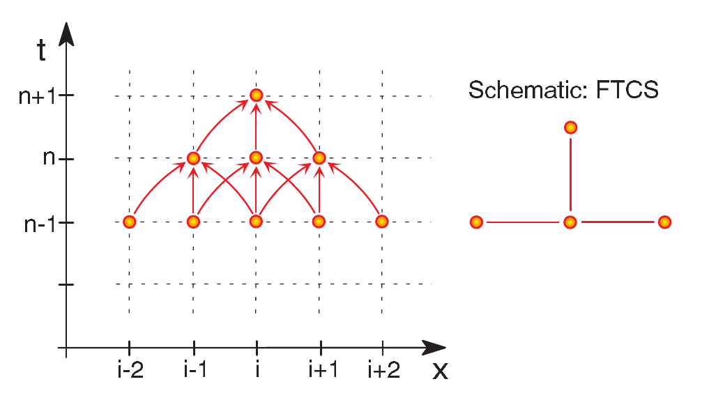
FTCS scheme.

4.5 Methods for diffusion equations: FTCS

• The amplification factor is \[ \xi(k)=1 -\frac{4\alpha \Delta t}{(\Delta x)^2}\sin(k\Delta x/2). \] leading to the stability criterion: \[ \frac{2\alpha\Delta t}{\Delta x}\leq 1 \hspace{0.3cm}\text{or}\hspace{0.3cm} s<1/2. \qquad(2)\] \(\Rightarrow\) the maximum allowed timestep is approx. the diffusion time across a cell of width \(\Delta x\).
• In general, the diffusion time across a spatial scale of size \(\lambda\) is \(\tau\sim\lambda^2/D\), which leads to a number of timesteps (based in Eq. Equation 2) of order \(\lambda^2/(\Delta x)^2\) …too many.

4.6 Methods for diffusion equations: Crank-Nicholson

• An idea to change the small CFL timestep of the diffusion eq. with the previous discretization is the Crank-Nicholson scheme, second-order accurate in time.
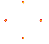
• Implicit Crank-Nicholson is based on a mixture of spatial derivatives using time levels \(n\) and \(n+1\) \[ \frac{f_j^{n+1} - f_j^{n}}{\Delta t} = \frac{\alpha}{2}L_{xx}(f_{j}^n + f_{j}^{n+1}) \] or \[ \frac{u_j^{n+1} - u_j^{n}}{\Delta t} = \frac{\alpha}{2}\left(\frac{(u_{j+1}^{n+1} -2u_j^{n+1} + u_{j-1}^{n+1}) +(u_{j+1}^{n} -2u_j^{n} + u_{j-1}^{n}) }{(\Delta x)^2} \right) \qquad(3)\]
• This scheme is unconditionally stable.

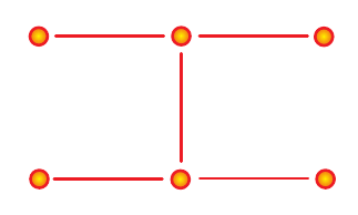
Crank-Nicholson scheme. The lines shows the derivatives. Horizontaly goes space, vertially time.

4.7 Methods for diffusion equations: Others

4.8 Methods for convection equations

4.9 Methods for convection equations

• The methods are hyperbolic PDEs, the prototype is \[ \frac{\partial f}{\partial t} + \frac{\partial f V}{\partial x}=0 \]

• Examples:

  • Mass continuity equation
  • Convection equation (from induction equation)
  • Some limits of the momentum equation (and Navier-Stokes equations). }

• Note: The system nonlinearity is cased by the convective acceleration term in the equations. The term represents an acceleration associated with the change in velocity with spatial position of the fluid element. Hence, any convective flow, whether turbulent or not, involves nonlinearity.

• An example of convective but laminar (nonturbulent) flow would be the passage of a viscous fluid (for example, oil) through a small converging nozzle. Such flows, whether exactly solvable or not, can often be thoroughly studied and understood.

4.10 Methods for convection equations

• Let us assume for simplicity \(V\) known and constant. This leads to the linear convection/advection equation: \[ \frac{\partial f}{\partial t} + V\frac{\partial f}{\partial x}=0 \] with solution \(f(x,t)=F(x-Vt)\), where \(F(x)=f(x,t=0)\).

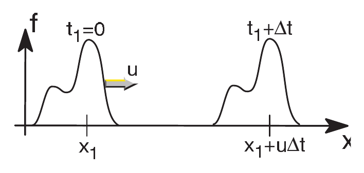
Solution of the linear convection equation, transport of the initial profile

4.11 Methods for convection equations: Upwind

• One the simplest first-order methods is the upwind scheme \[ \frac{f_{j}^{n+1} - f_{j}^{n}}{\Delta t} + V\frac{f_{j}^{n} - f_{j-1}^{n}}{\Delta x}=0 \] yielding the algebraic equation \[ f_j^{n+1} = (1-c)f_j^{n} + c f_{j-1}^{n} \]
• Stability requires \(c=V\Delta t/\Delta x \leq 1\) (CFL condition: information should travel at most one grid spacing in a single time step)

Upwind scheme

4.12 Methods for convection equations: Leapfrog

• One of the simplest 2nd order schemes for convection eqs is Leapfrog: \[ \frac{f_j^{n+1} - f_j^{n-1}}{2 \Delta t} + \frac{V}{2 \Delta x}(f_{j+1}^{n} - f_{j-1}^{n})=0 \] yielding the algebraic eq: \[ f_j^{n+1} = f_j^{n-1} - c (f_{j+1}^{n} - f_{j-1}^{n}) \] with \(c=V\Delta t/\Delta x\).

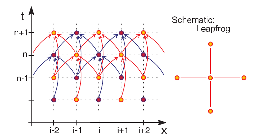
Leapfrog scheme

4.13 Methods for convection equations: Leapfrog

• Note that the leapfrog scheme for ODEs, where velocities are calculated at half-timesteps, can also be written in terms of quantities defined only at integer time steps like above.
• Stable for \(c<1\), with \(c=V\Delta t/\Delta x\). No diffusion.
• Because the grids associated to odd and even points are independent, solutions can develop independently and lead to strong oscillations on the grid scale.

4.14 Methods for convection equations: Lax-Wendroff

• Another popular scheme is Lax-Wendroff, which uses a forward time-discretization plus a correction that eliminates the lowest order error. \[ \frac{\partial f}{\partial t}\approx \frac{f_j^{n+1}-f_j^{n}}{\Delta t} - \frac{\Delta t}{2}\frac{\partial^2 f}{\partial t^2}= \frac{f_j^{n+1}-f_j^{n}}{\Delta t} - \frac{\Delta t }{2}V^2\frac{\partial^2 f}{\partial x^2} \] yielding the algebraic eq: \[ f_j^{n+1} = f_j^{n} - \frac{c}{2}(f_{j+1}^{n} - f_{j-1}^{n})+\frac{c^2}{2}(f_{j+1}^{n} - 2f_{j}^{n} + f_{j-1}^{n}) \qquad(4)\] with \(c=V\Delta t/\Delta x\).
• To minimize errors due to not constant \(V\) or \(\Delta X\), this is usually implemented as a two-step method: \[ f_{j+1/2}^{*} = \frac{1}{2}(f_{j+1}^{n} - f_{j}^{n})+\frac{c}{2}(f_{j+1}^{n} - f_{j}^{n}) \\ f_{j}^{n+1} = f_j^n + \frac{c}{2}(f_{j+1/2}^{*} - f_{j-1/2}^{*}) \]
• This scheme is also stable for \(c<1\)

4.15 Methods for convection equations: Dissipation

• Any numerical discretization of the convection equations generally introduces numerical dispersion and diffusion.
• Numerical dispersion (depends on the odd spatial derivatives): wave propagation speed can become dependent on the wave number and deviating from the physical propagation speed, which affect the transport of physical quantities like mass, momentum and energy
• Numerical diffusion (depends on the even spatial derivatives) leads to damping of waves or diffusion of density. Diffusion of pressures/temperatures implies conduction of heat.
• One way to correct for those effects is by adding corrective terms, which eliminate the dominant order terms for diffusion and convection, equivalent to introduce higher order methods.
• Those effects are better analyzed in the Fourier space.

4.16 Methods for convection equations: Dissipation

• Note that the Lax-Wendroff scheme is a finite difference representation of : \[ \frac{\partial f}{\partial t} + V\frac{\partial f}{\partial x} = \xi \frac{\partial^2 f }{\partial x^2} + \zeta \frac{\partial^3 f }{\partial x^3} \qquad(5)\] which is a advection-diffusion equation plus higher-order derivative terms with \[ \xi=\frac{c V}{2}\frac{\Delta x^2}{2}\;\;\;\;\;\;\;\;\zeta=\frac{-V\Delta x^2}{6}(1-\alpha^2) \] implying a diffusion time-scale \(\tau\approx \lambda^2/\xi\).
• A similar analysis for the upwind scheme results in a second order finite difference representation of a similar advection-diffusion equation with a dissipative term \[ \xi=\frac{V \Delta x}{2} \]
• A more accurate numerical scheme is not necessarily better.

4.17 Methods for convection equations: Others

4.18 Methods for transport equations

4.19 Methods for transport equations

• A PDE combining convection and diffusion is usually called a transport equation \[ \frac{\partial f}{\partial t} + V\frac{\partial f}{\partial x} - \alpha \frac{\partial^2 f}{\partial x^2} =0 \]
• For steady state, one can compare the order of magnitude of the convection and diffusion terms, yielding: \(L_0=\alpha/V\). For \(L<(>)L_0\) diffusion (convection) term dominates
• Cell Reynolds number: \[ R_{cell}=\frac{\Delta x}{L_0}=\frac{V\Delta x}{\alpha}=\frac{\tau_{diff}}{\tau_{conv}} \] where \(\tau_{diff}=\Delta x^2/\alpha\) and \(\tau_{conv}=\Delta x/V\)
• In order for the solution to resolve the relevant physics, \(R_{cell}<1\).
• An explicit method should resolve both the diffusion time (\(s=\alpha\Delta t/\Delta x^2\leq 1\)) and the convection time (\(c=V\Delta t/\Delta x \leq 1\)). V can be either a convection velocity or a typical wave speed.

4.20 Methods for transport equations: FTCS

• The forward time central space scheme is: \[ \frac{f_j^{n+1} - f_j^{n}}{\Delta t} = -\frac{V}{2 \Delta x}(f_{j+1}^{n} - f_j^{n}) +\frac{\alpha}{\Delta x^2}(f_{j-1}^{n} - 2f_j^{n} + f_{j+1}^{n}) \] giving the algebraic eq: \[ f_j^{n+1} = (s+c/2)f_{j-1}^{n} + (1-2s)(f_{j}^{n}) + (s-c/2)f_{j+1}^{n} \] with \(c=V\Delta t/\Delta x\) and \(s=\alpha\Delta t/\Delta x^2\).
• FTCS leads to a stable scheme for this transport eq, while for convection eqs. is unstable.
• For accuracy this scheme requires: \[ R_{cell}=c/s\ll 2/c \]

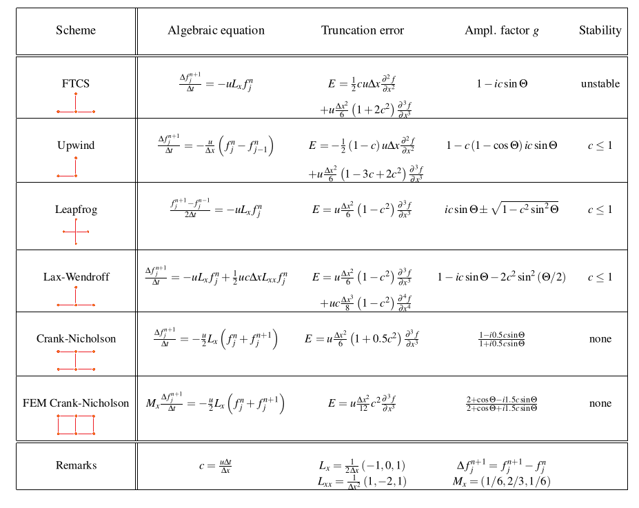
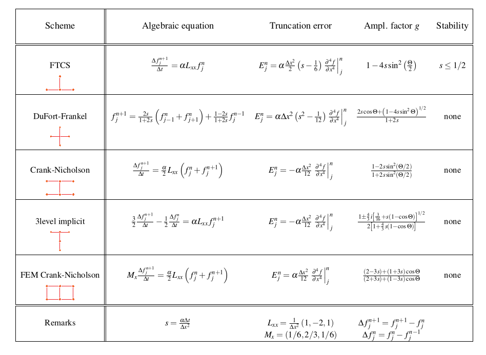
4.21 Methods for transport equations: Summary

Dufort-Frankel scheme.

4.22 Non-linear transport equations

• The prototype is Burgers equation: \[ \frac{\partial V}{\partial t} + V\frac{\partial V}{\partial x} - \nu \frac{\partial^2 V}{\partial x^2} =0 \]
• Nonlinear term is \(V\frac{\partial V}{\partial x}\), and the term including \(\nu\) is the viscous term.
• The conservative form is written with the second term as \(\partial F/\partial x\), with \(F=V^2/2\).
• Wave steepening and breaking: wave speed depends on the amplitude or other parameters.
• Examples: sound waves (depending on the temperature/pressure), shock waves (amplitude), tsunamis (amplitude depending on the depth of the water).

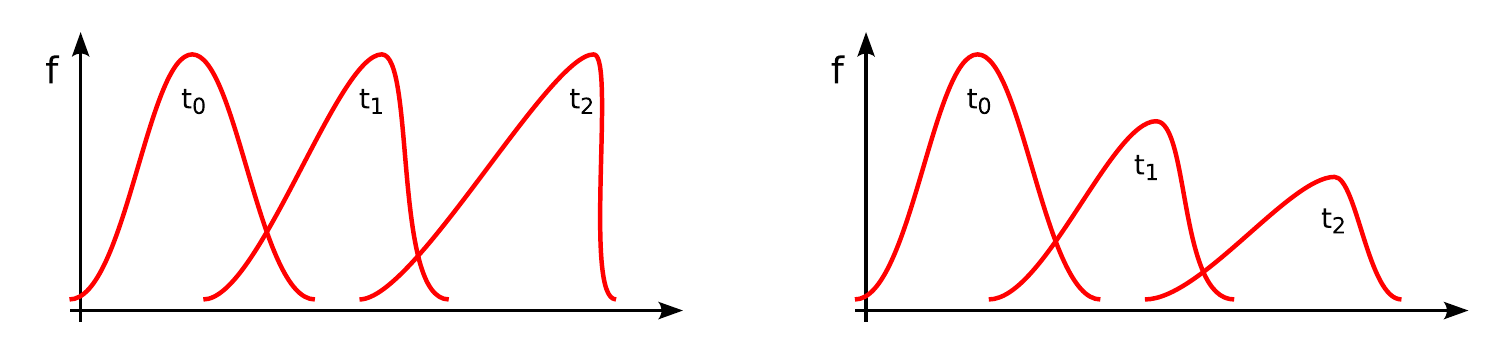
Solution of the Burgers equation. Left: Inviscid case (\(\nu=0\)). Right: Viscous medium

4.23 Methods for elliptic equations

4.24 Solution methods for elliptic PDEs

• They arise mostly as steady-state limits of some hyperbolic or parabolic equations:
  • Incompressible flow problems
  • Grad-Shrafanov equation (equilibrium 2D MHD equations). \(\nabla^2A=-\mu_0(d/dA)(p + B_z^2/2\mu_0)\)
  • Some formulations of time-dependent MHD equations in terms of potentials \(A\) and \(\psi\)
  • Darwin approximation of the Vlasov-Maxwell system of eqs (no light waves).
  • But the standard prototype is the Poisson or Laplace equations

4.25 Solution methods for elliptic PDEs

• 2D Poisson eq \[ \frac{\partial^2 u}{\partial x^2} + \frac{\partial^2 u}{\partial y^2} = R(x,y) \qquad(6)\] with Dirichlet BCs: \(u(0,y)\), \(u(L,y)\) (\(0<y<L\)) \(u(x,0)\), \(u(x,L)\) (\(0<x<L\))

  The 2nd order finite difference eq (derived by a Taylor expansion) is \[ u_{j+1,k} + u_{j-1,k} + u_{j,k+1} + u_{j,k-1} - 4u_{j,k} = \Delta x^2 R_j,k \] {#eq-poisson_diff) Let the \((N+1)^2\) vector of unknowns be denoted by \(\vec{X}\). The matrix form of eq. ?@eq-poisson_diff is \(\bar{A}\cdot\vec{X}=\vec{b}\)

4.26 Solution methods for elliptic PDEs

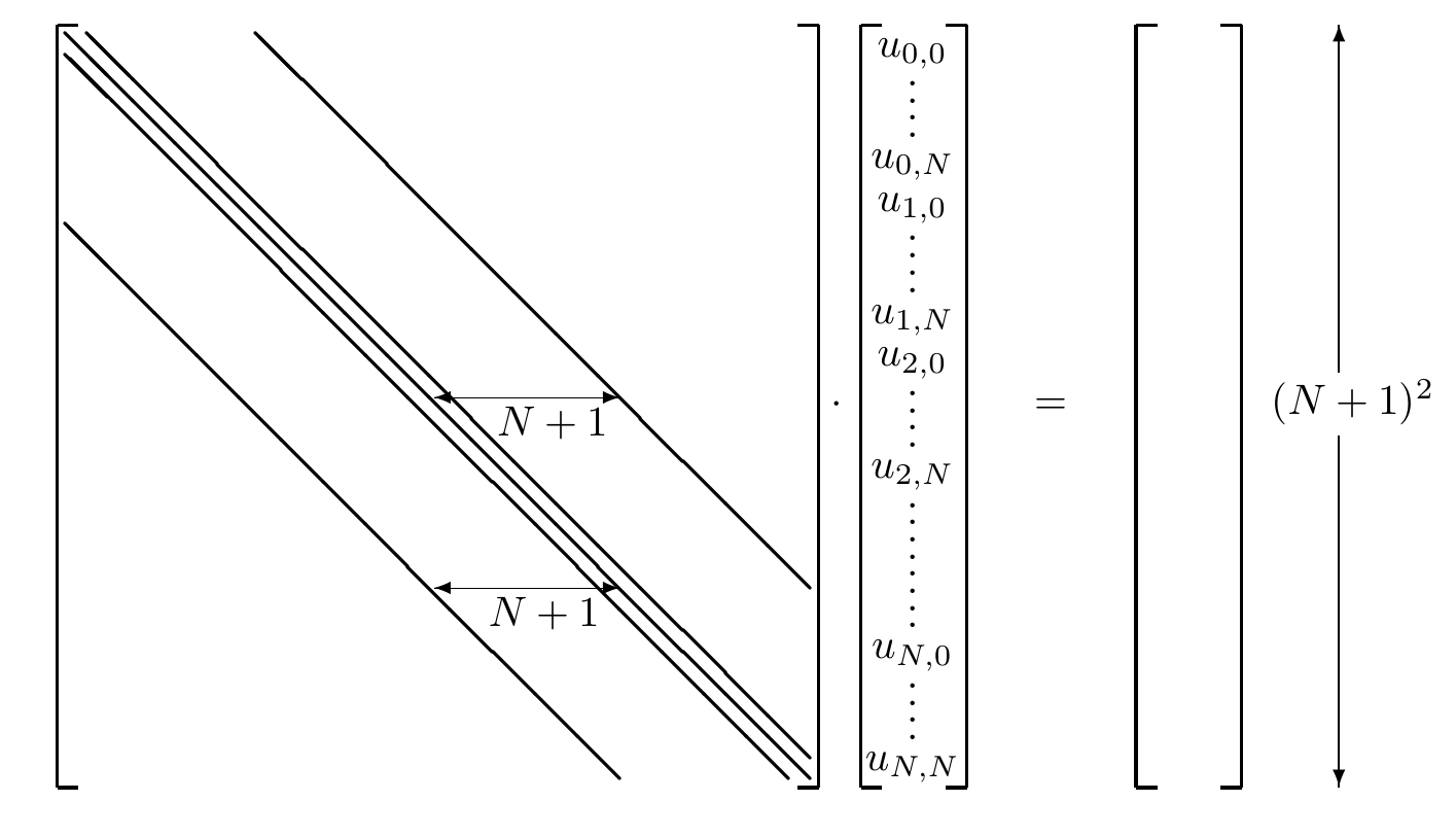
Sparse matrix \(\bar{A}\)

This matrix eq. must be inverted to solve for the unknowns (although the actual inverse is not normally calculated). Some methods are:

• Direct invertion using Gauss or LU decomposition
• Direct inversion using block tridiagonal methods
• Iterative methods (multigrid, Krylov space methods). A physical approach involves adding time derivatives terms (converting it to parabolic/hyperbolic eqs), and advancing it in time until a steady state is obtained.
• Direct methods based on transform techniques (e.g.: Fourier)}

4.27 Multigrid methods

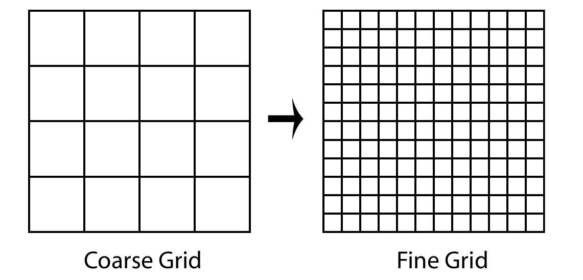
Schematics of multigrid method

• Iterative methods benefit greatly from a good initial guess: A coarse grid solution can be used to initialize a finer grid iteration
• On a given grid, the short wavelengths components of the error decay much faster than the long wavelengths. So, the coarse mesh is more efficient in handling long components of the error but the fine mesh is needed for the short wavelength components.
• The error satisfies the same matrix eqs. as the unknown.
• Two basic steps: nested iteration (for the initial guess), coarse grid correction.

4.28 Fast Fourier methods

• Fourier (spectral) methods can be applied to solve boundary problems (e.g.: elliptic eqs,) that lead to large sparse linear systems of the form \(\bar{A}\cdot\vec{x}=\vec{b}\)
• The algorithm is based on a Fast Fourier transform (FFT), a clever trick to avoid the calculation of \(N^2\) multiplications and \(N(N-1)\) that are required for a direct finite Fourier transform. Instead, if \(N\) is equal to a power of 2, it leads to a product of \(log_2(N)\) sparse matrices.
• It works best when the PDE has constant coefficients and the boundaries coincide with the coordinate lines.

5 System of fluids/MHD equations

5.1 General algorithms

5.2 Fluid equations

• In fluid dynamics, we can write the equations for conservation of mass, momentum and energy as: \[ \frac{\partial\vec{q}}{\partial t} + \frac{\partial \bar{F}}{\partial x}= 0 \qquad(7)\] with \(\vec{q}\) and \(\bar{F}\) in 1D defined as \[ \vec{q}= \begin{pmatrix} \rho, & \rho V, & P/(\gamma -1) + (1/2)\rho V^2\end{pmatrix}^T\\ \vec{F}= \begin{pmatrix} \rho V, & \rho V^2 + P, & (\gamma P/(\gamma -1) + (1/2)\rho V^2)V \end{pmatrix}^T \] in 3D, \(\bar{F}\) is a 3x5 matrix (3 dimensions + 5 dependent variables, \(\rho\), \(P\), \(\vec{V}\))
• In many practical cases dissipative terms can be added to the terms in \(\bar{F}\), proportional to the derivatives \(\partial/\partial x\).
• MHD equations have the same structure with the additional equation and terms for the magnetic field.

5.3 MHD equations in conservative form

Conservative form of the MHD equations

\[ \frac{\partial \rho}{\partial t}= -\nabla \cdot\rho\vec{V} \\ \frac{\partial \rho \vec{V}}{\partial t}= -\nabla \cdot \left[\rho\vec{V}\vec{V} + \left(P + \frac{B^2}{2\mu_0}\right)\vec{1} - \frac{\vec{B}\vec{B}}{\mu_0}\right] \\ \frac{\partial \vec{B}}{\partial t} = \nabla\times\left[\vec{V}\times\vec{B}-\eta\vec{J}\right]\\ \frac{\partial w}{\partial t} = -\nabla \cdot \left[ \vec{V}\cdot\left(w + \left(P + \frac{B^2}{2\mu_0}\right) \right) -\frac{1}{\mu_0}(\vec{V}\cdot\vec{B})\vec{B} + \eta \vec{J}\times\vec{B} \right] \]

where the electric field, current density and total energy density are: \[ \vec{E} = - \vec{V}\times\vec{B} + \eta\vec{J} \\ \vec{J} = \nabla\times\vec{B}/\mu_0\\ w = \frac{1}{2}\rho V^2 + \frac{1}{2\mu_0} B^2 + \frac{P}{\gamma -1} \] \(\gamma=5/3\). Typical speeds: sound speed \(c_s=\sqrt{\gamma P/\rho}\), Alfv'en speed \(V_A=B/\sqrt{\mu_0 \rho}\).

5.4 Discretization for fluid equations

• Leapfrog: \[ \vec{q}_j^{n+1} = \vec{q}_j^{n-1} - \frac{\Delta t}{2\Delta x}(\vec{F}_{j+1}^n - \vec{F}_{j-1}^n) \]
• Lax-Wendroff: \[ \vec{q}_{j+1/2}^{*} = \frac{1}{2}\left(\vec{q}_j^{n} + \vec{q}_{j+1}^{n}\right) - \frac{\Delta t}{2\Delta x}(\vec{F}_{j+1}^n - \vec{F}_{j}^n)\\ \vec{q}_{j}^{n+1} = \vec{q}_j^{n-1} - \frac{\Delta t}{\Delta x}( \vec{F}_{j+1/2}^*-\vec{F}_{j-1/2}^*) \]
• Implicit scheme: Crank-Nicholson \[ \vec{q}_j^{n+1} - \vec{q}_j^{n} = - \frac{\Delta t}{4\Delta x}\left[ (\vec{F}_{j+1}^n - \vec{F}_{j-1}^n) + (\vec{F}_{j+1}^{n+1} - \vec{F}_{j-1}^{n+1}) \right] \]
• Note that all those schemes are 2nd order. Since dissipative terms involve second order derivatives, they should be treated via non-linear transport method or other discretizations for parabolic equations (e.g. DuFort-Frankel).

5.5 Methods for diffusion equations: Dufort-Frankel

• The Dufort-Frankel scheme is based on a modification of the FTCS scheme for the diffusion (parabolic) equation by using centered difference in time and the middle term in the Laplacian (\(2f_{j}^n\)) split into two time levels: \[ \frac{f_j^{n+1} - f_j^{n-1}}{2\Delta t} = \frac{\alpha}{\Delta x^2} L_{xx} f_j^n=\frac{\alpha}{\Delta x^2}(f_{j-1}^n - (f_{j}^{n-1} + f_{j}^{n+1}) + f_{j+1}^n ) \] and rearranging: \[ f_j^{n+1} = \frac{2s}{1+2s}(f_{j-1}^n + f_{j+1}^n ) + \frac{1-2s}{1+2s}f_{j}^{n-1} \]
• This scheme is unconditionally stable.

5.6 Flux conserving algorithms

• Grid points are considered cell centers at \(x_i\) (\(i=1,..N\)), while cell interfaces located at \(x_{i+1/2}=(x_i+x_{i+1})/2\) (\(N\) cell centers and \(N-1\) cell interfaces)
• We could consider the boundaries at \(x_{1/2}\) and \(x_{N+1/2}\), making a total of \(N+1\) cell interfaces.
• Let consider a 3D situation with the volume of each cell \(V=\Delta x S\) and \(S=\Delta y \Delta z\).
• the conserved quantity is \(q_i^N\), the total content in each cell is \(Q_i^n=q_i^n V\)
• Any change in the conserved \(Q_i^n\) must come from inflows and outflows through the cell interfaces via a flux \(f\): \[ \frac{dQ_i}{dt}\approx \frac{Q_i^{n+1} - Q_i^{n}}{\Delta t} =(f_{i-1/2}^{n+1/2} - f_{i+1/2}^{n+1/2})S \]
• Using the definitions of \(S\) and \(Q_i\), we get: \[ \frac{q_i^{n+1} - q_i^{n}}{\Delta t} =\frac{f_{i-1/2}^{n+1/2} - f_{i+1/2}^{n+1/2}}{\Delta x} \]
• The different flux conserving algorithms differ only in the calculation of \(f_{i\pm1/2}^{n+1/2}\) in terms of \(q_{i\pm}^{n}\) (e.g., Donor-cell advection, piecewise linear schemes, flux-limiter methods), and the methods are usually called Finite Volume Methods.

5.7 Finite Volume Methods

• Those methods are not applied to the equations in conservation form, but rather on their integral form.
• The computational domain is subdivided into a finite number of contiguous volumes (e.g.: cuboids) and the quantities are calculated at the centroid.
• The surfaces of those volume are used for the integral conservation relations, while derivatives are transformed via Gauss divergence theorem.
• Example: \[ \left( \frac{\partial \phi}{\partial x}\right)= \frac{1}{\Delta V}\int_{\Delta V} \frac{\partial \phi}{\partial x}d^3x=\frac{1}{\Delta V}\int_{\partial V}\phi dS^x\approx \frac{1}{\Delta V}\sum_{j=1}^N \phi_j S_j^x \] where \(\phi_j\) are the values of the function at the surfaces and \(N\) is the number of bounding surfaces of the volume.

5.8 Properties

5.9 Hyperbolic character of the ideal MHD equations

Advective form of the MHD equations

\[ \frac{\partial \rho}{\partial t} + \vec{V}\cdot\nabla\rho + \rho \nabla \cdot \vec{V}=0 \\ \frac{\partial \vec{V}}{\partial t} + \vec{V}\cdot\nabla\vec{V} + \frac{\nabla P}{\rho} =0 \\ \frac{\partial P}{\partial t} + \vec{V}\cdot\nabla P + \gamma P\nabla\cdot\vec{V} =0 \\ \frac{\partial \vec{B}}{\partial t} + \vec{V}\cdot\nabla\vec{B} - \vec{B}\cdot\nabla\vec{V} + \vec{B}(\nabla\cdot\vec{V}) =0 \]

Those equations can be expressed as: \[ \frac{\partial \vec{q}}{\partial t} + \bar{A}_i\frac{\partial \vec{q}}{\partial x_i}=0 \qquad(8)\]

5.10 Hyperbolic character of the ideal MHD equations

• With \[ \vec{q}= \begin{pmatrix} \rho, P , V_x, V_y, V_z, B_x, B_y, B_z \end{pmatrix}^T\\ \bar{A}_x = \begin{pmatrix} V_x & 0 & \rho & 0 & 0 &0 & 0& 0\\ 0 & V_x & \gamma\rho & 0 & 0 &0 & 0& 0 \\ 0 & 1/\rho & V_x & 0 & 0 & 0 & B_y/(\mu_0\rho) & B_z/(\mu_0\rho) \\ 0 & 0 & 0 & V_x & 0 & 0 & -B_x/(\mu_0\rho) & 0 \\ 0 & 0 & 0 & 0 & V_x & 0 & 0 & -B_x/(\mu_0\rho) \\ 0 & 0 & 0 &0 & 0& V_x & 0& 0\\ 0 & 0 & B_y & -B_x & 0 & 0& V_x & 0\\ 0 & 0 & B_z & 0 & -B_x & 0& 0 & V_x \end{pmatrix} \]
• The determinant is: \[ {\rm det}(\bar{A}_x - v\vec{I})= (v - V_x)^2 \left[ (v - V_x)^2 - V_{Ax}^2\right ] \left[ (v - V_x)^4 - (c_s^2 + V_{A}^2)(v-V_x)^2 + C_s^2 V_{Ax}^2\right ] \]
• The system is because the eigenvalues of \(\bar{A_i}\vec{n}_i\) are real for any unit vector \(\vec{n}\) and linearly independent.

5.11 Hyperbolic character of the ideal MHD equations

• The eigenvalues of the previous equations can be identified as wave speeds, and the eigenvectors as wave modes, and \(\vec{n}_i\) the unit wave vector normal to the wavefronts.
• Two modes with \(v=V_x\), do not propagate. One is an entropy wave involving a density perturbation only, and the other is an unphysical perturbation of \(\nabla \cdot\vec{B}\).
• Alfv'en waves with speed \(V_x\pm V_{Ax}\).
• Fast and slow magnetoacoustic/magnetosonic waves (combining \(c_s\) and \(V_{A}\)).

5.12 Stability of discretized MHD equations

• Von Neumann stability methods is only applicable to linear system of eqs. \(\eqref{zeroform}\), and therefore the fluid or MHD equations have to be linearized.
• After some tedious calculations, the discretization of the system of equations leads to: \[ \vec{q}_{j}^{n+1} = \bar{G}\vec{q}_{j}^{n} \]
• Any amplification of any \(\vec{q}_{j}\) component leads to an exponential growth. More precisely, any instability exists if any eigenvalue of the matrix \(\bar{G}>1\).
• Stability analysis is usually carried out for homogeneous system. For inhomogeneous system the more stringent stability conditions apply at the locations of the most severe restrictions (largest speeds, etc).

5.13 Stability of discretized MHD equations

Stability analysis leads to three different requirements: 1. Hyperbolic part: maximum velocity for information transport: either faster wave speed \(c_{max}\) and the maximum convective velocity \(v_{max}\): \[ \Delta t \leq \frac{\Delta x}{|c_{max} + v_{max}|} \] 2. Parabolic part: Diffusive or viscous time across a cell. For example, for the FTCS scheme with a diffusion coefficient \(\alpha\) \[ \alpha\Delta t/\Delta x^2<1/2 \] 3. Source terms in conservation eqs, due to, e.g., ionization, recombination, or (chemical) production rates. For example: \[ \frac{\partial \rho}{\partial t} + \nabla\cdot(\rho\vec{V})=\nu_s (\rho_s - \rho) \] which implies \(\nu_s\Delta t \leq 1\)

5.14 Symmetries of the ideal MHD equations

• Translations of time and space, and rotations of space. Via Noether’s theorem they are related to conservation of energy, momentum and angular momentum.
• Reversal of time: related to absence of dissipation
• Reflections of space (except \(\vec{B}\) which is a pseudovector)
• Galilean transformations
• Reversal of sign of \(\vec{B}\)
• Similarity transformations: if space and time are rescaled by the following factors \[ \vec{x}\to \lambda \vec{x},\hspace{1cm}, t\to \mu t \] then \[ \vec{V}\to \lambda\mu^{-1}\vec{V},\;\; \rho \to \mu^{-2}\rho,\;\; P \to \lambda^2 \mu^{-4} P \;\; \vec{B}\to \lambda\mu^{-2}\vec{B} \]

5.15 Others

5.16 Boundary conditions and ghost cells

• Some typical boundary conditions, for 1D case, left boundary and the fluid variables \(\rho\) and \(V\)
  1. Periodic BCs: \(\rho[0]=\rho[N_x], V[0]=V[N_x]\)
  2. Reflective BCs: \(\rho[0]=\rho[1], V[0]=-V[1]\)
  3. Free outflow/inflow: \(\rho[0]=\rho[1], V[0]=V[1]\)
  4. Free outflow, no inflow, \(\rho[0]=\rho[1], V[0]=-{\rm abs}(V[1])\)
  5. Given time-dependent BC: \(\rho[0]=\rho(t), V[0]=V(t)\)

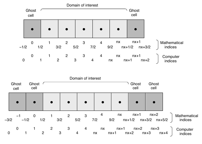
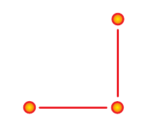
5.17 Ghost cells

• Example for a flux-conserving algorithm with three point stencil (top) and 4-5 point stencil (bottom).

5.18 Divergence of magnetic field

• One of the major issues in MHD codes (in contrast to the pure HD fluid system of eqs.) is possible deviations from \(\nabla\cdot\vec{B}=0\) due to discretization errors
• Divergence cleaning: The perhaps simplest approach is to correct the deviations from the magnetic field with a finite divergence \(\vec{B}'\) by solving a Poisson equation in order to obtain a “cleaned” \(\vec{B}\) \[ \nabla^2\phi = \nabla\cdot\vec{B}'\\ \vec{B} = \vec{B}'- \nabla\phi \]
• Other approaches are based on finite volume discretizations of the MHD equations, like the constrained transport method Evans and Hawley (1988).

5.19 Tutorial for HD

• VorteGrid: Interactive Fluid Simulation for Games and Movies {https://www.mijagourlay.com/fluid}
• https://web.archive.org/web/20191104194657/https://software.intel.com/en-us/articles/fluid-simulation-for-video-games-part-1/

5.20 Popular astrophysical MHD codes

• Pencil: https://github.com/pencil-code/pencil-code
• ENZO: https://github.com/enzo-project/enzo-dev, Bryan et al. (2014)
• ATHENA++: https://github.com/PrincetonUniversity/athena, James M. Stone et al. (2008),James M. Stone et al. (2020)
• RAMSES: https://bitbucket.org/rteyssie/ramses/wiki/Home, Masson et al. (2012)
• NIRVANA: https://gitlab.aip.de/ziegler/NIRVANA Ziegler (2008)
• PLUTO: http://plutocode.ph.unito.it, Mignone et al. (2012)
• MPI-AMRVAC 2.0: https://github.com/amrvac/amrvac, Xia et al. (2018)
• CRONOS: https://www.uibk.ac.at/astro/research_groups/ralf-kissmann/home/cronos-code.html, Kissmann et al. (2018)

5.21 References

Baumjohann, Wolfgang, and Rudolf A Treumann. 1997. Basic Space Plasma Physics. Imperial College Press ; Distributed by World Scientific Pub. https://doi.org/10.1142/p015.

Bittencourt, J. A. 2004. Fundamentals of Plasma Physics. Springer.

Bryan, Greg L, Michael L Norman, Brian W. O’Shea, Tom Abel, John H Wise, Matthew J Turk, Daniel R Reynolds, et al. 2014. “ENZO: AN ADAPTIVE MESH REFINEMENT CODE FOR ASTROPHYSICS.” Astrophys. J. Suppl. Ser. 211 (2): 19. https://doi.org/10.1088/0067-0049/211/2/19.

Cravens, T. 1997. Physics of solar system plasmas. Cambridge University Press.

Evans, Charles R., and John F. Hawley. 1988. “Simulation of magnetohydrodynamic flows - A constrained transport method.” Astrophys. J. 332 (9): 659. https://doi.org/10.1086/166684.

Kissmann, R., J. Kleimann, B. Krebl, and T. Wiengarten. 2018. “The CRONOS Code for Astrophysical Magnetohydrodynamics.” Astrophys. J. Suppl. Ser. 236 (2): 53. https://doi.org/10.3847/1538-4365/aabe75.

Masson, J, R Teyssier, C. Mulet-Marquis, P Hennebelle, and G Chabrier. 2012. “INCORPORATING AMBIPOLAR AND OHMIC DIFFUSION IN THE AMR MHD CODE RAMSES.” Astrophys. J. Suppl. Ser. 201 (2): 24. https://doi.org/10.1088/0067-0049/201/2/24.

Mignone, A, C Zanni, P Tzeferacos, B. van Straalen, P Colella, and G Bodo. 2012. “THE PLUTO CODE FOR ADAPTIVE MESH COMPUTATIONS IN ASTROPHYSICAL FLUID DYNAMICS.” Astrophys. J. Suppl. Ser. 198 (1): 7. https://doi.org/10.1088/0067-0049/198/1/7.

Stone, James M, Thomas A Gardiner, Peter Teuben, John F Hawley, and Jacob B Simon. 2008. “Athena: A New Code for Astrophysical MHD.” Astrophys. J. Suppl. Ser. 178 (1): 137–77. https://doi.org/10.1086/588755.

Stone, James M., Kengo Tomida, Christopher J. White, and Kyle G. Felker. 2020. “The Athena++ Adaptive Mesh Refinement Framework: Design and Magnetohydrodynamic Solvers.” The Astrophysical Journal Supplement Series 249 (1): 4. https://doi.org/10.3847/1538-4365/ab929b.

Winske, D., and N. Omidi. 1996. “A nonspecialist’s guide to kinetic simulations of space plasmas.” J. Geophys. Res. 101 (A8): 17287. https://doi.org/10.1029/96JA00982.

Xia, C., J. Teunissen, I. El Mellah, E. Chané, and R. Keppens. 2018. “MPI-AMRVAC 2.0 for Solar and Astrophysical Applications.” Astrophys. J. Suppl. Ser. 234 (2): 30. https://doi.org/10.3847/1538-4365/aaa6c8.

Ziegler, U. 2008. “The NIRVANA code: Parallel computational MHD with adaptive mesh refinement.” Comput. Phys. Commun. 179 (4): 227–44. https://doi.org/10.1016/j.cpc.2008.02.017.