Lecture 1: Introduction to astrophysical simulations
October 17, 2024
2.1 Plasma phenomenology
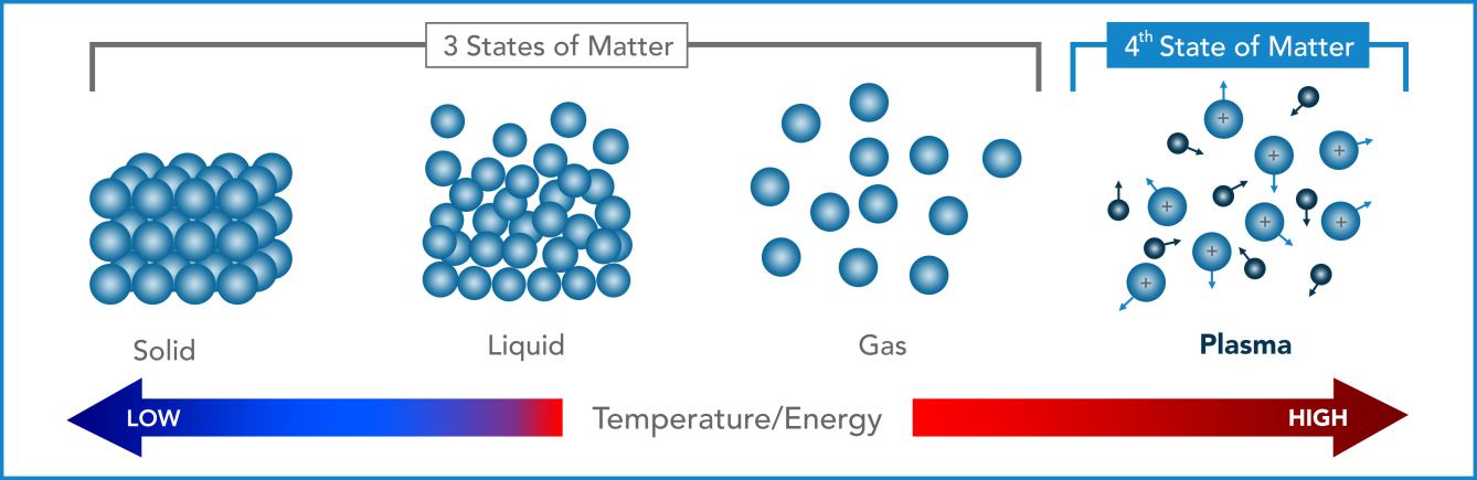
- Partially or fully ionized (Saha equation)
- High electrical conductivity
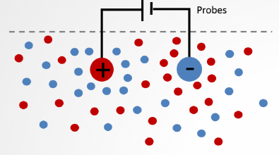
- Quasi-neutral
- Collective behaviour
- Magnetic forces
2.2 Plasmas on Earth
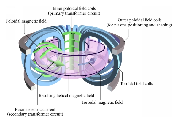
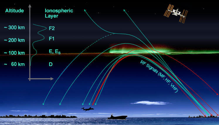
2.3 Earth’s ionosphere
2.4 Earth’s aurora
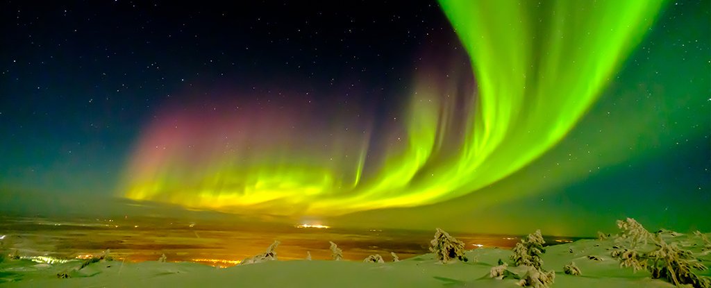
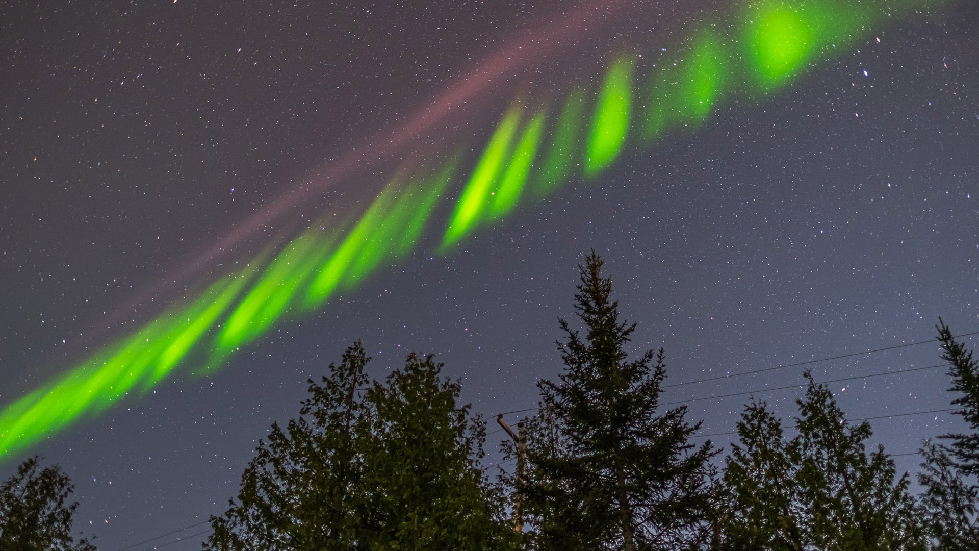
Credit: Space.com
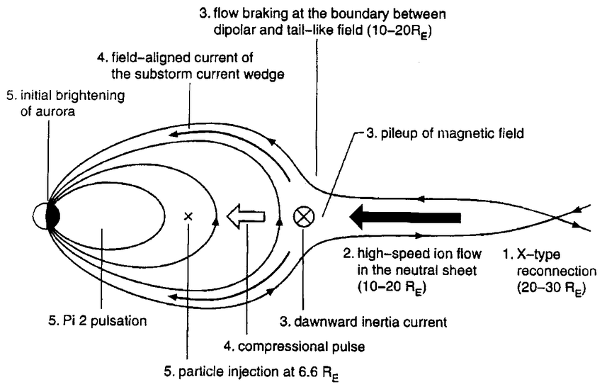
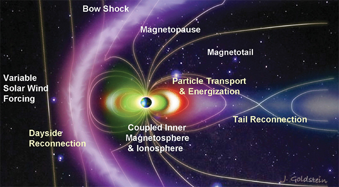
2.5 Earth’s magnetosphere
2.6 From the Sun to the Earth
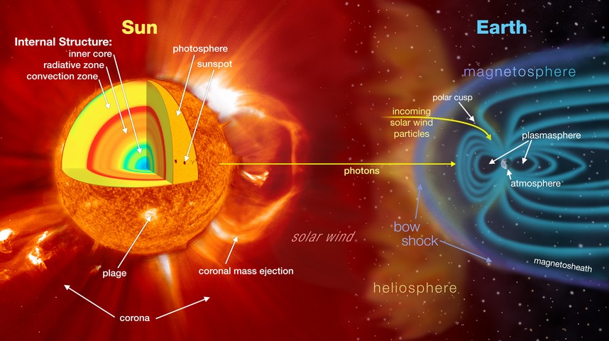
2.7 Sun/Stars
- Solar photosphere
- Solar atmosphere: Chromosphere, Corona.
![]()
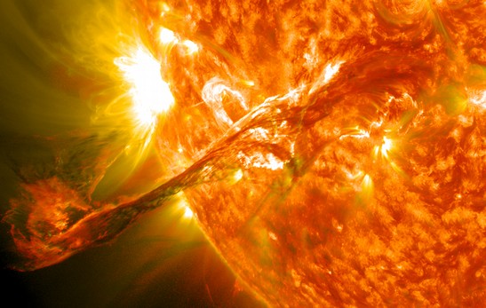
CME eruption on the Sun (SDO)
2.8 Comets
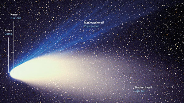
Comet Hale Bopp 1997
2.9 Interstellar medium (ISM)

Star formation regions in the Large Magellanic Cloud
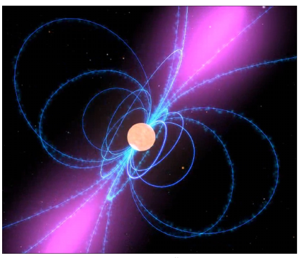
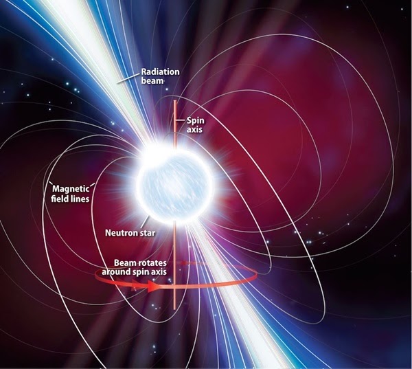
2.10 Pulsar magnetospheres
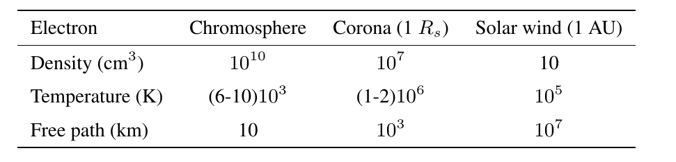
4.1 Plasma parameters
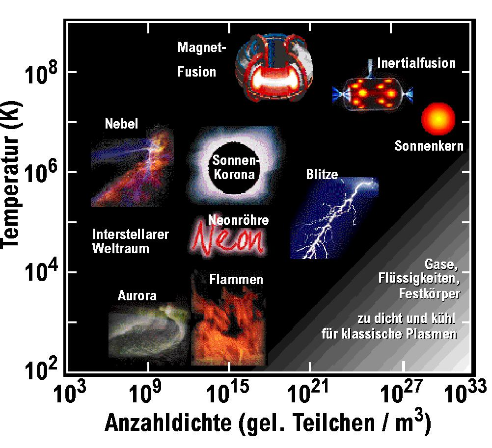
- Temperature
- Number density
- Magnetic field (not in the figure)
- Cold plasmas
- Hot plasmas
4.2 Collisions in plasmas
- Plasmas can be partially or fully ionized.
- Scattering is different: collisions among and with neutrals: large angle scattering.
- Charged particles: smooth small angle scattering only.
- Collisions enforce thermal equilibrium.
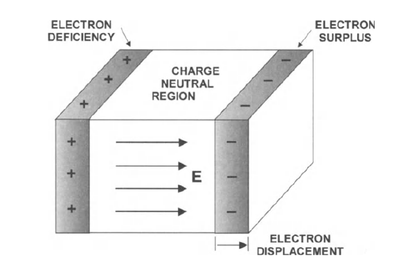
4.3 Length scales: Debye length
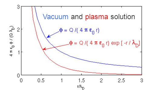
- The Coulomb potential of each particle is shielded by other charges \[\phi_D=\frac{q}{4\pi\epsilon_0 r}\exp\left(-\frac{r}{\lambda_{De}}\right).\]
- The electrostatic potential is screened out on distances larger than the Debye length \[ \lambda_{De} = \sqrt{\frac{\epsilon_0 k_B T_e}{n_e e^2}}. \]
- The plasma is quasi-neutral only for distances \(L\gg \lambda_{De}\).
- At sub-Debye length scales, charge separation occurs.
- An ideal plasma must have a sufficient number of particles in a Debye sphere to enforce their collective behavior. Plasma parameter \[ N_D=n_e \left( \frac{4}{3}\pi \right)\lambda_{De}^3 \gg 1. \]
4.4 Time scales: Plasma frequency
- Plasma frequency \[ \omega_{pe}=\sqrt{\frac{n_e e^2}{\epsilon_0 m_e}}. \]
- Typical response of electrons to restore quasineutrality when disturbed by external forces.
- Note that \[ \omega_{pe}= \frac{v_{th,e}}{\lambda_{De}}=\frac{\sqrt{\frac{k_BT_e}{m_e}}}{\lambda_{De}}. \]
- Collective behaviour
4.5 Time scales: Magnetic field and gyromotion
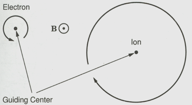
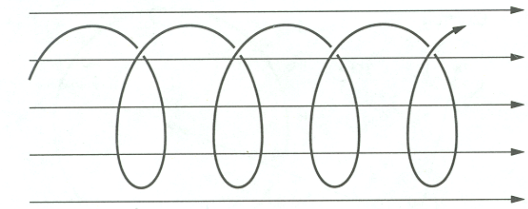
- Single particle motion and Lorentz force \[ m\frac{d\vec{v}}{dt}=q\vec{v}\times\vec{B} \]
- Gyro/cyclotron/Larmor-frequency \[ \Omega_c=\frac{qB}{m} \]
- Gyro/Larmor-radius \[ \rho=\frac{|v_{\perp}|}{\Omega_c}=\frac{m|v_{\perp}|}{|q|B} \] (usually \(|v_{\perp}|=v_{th}\)).
- Ratio of thermal to magnetic pressure. Plasma-\(\beta\) \[ \frac{nk_BT}{\frac{B^2}{2\mu_0}} \propto \left(\frac{\omega_{pe}}{\Omega_{ce}}\right)^2\left(\frac{v_{th}}{c}\right)^2. \]
4.7 Plasma parameters
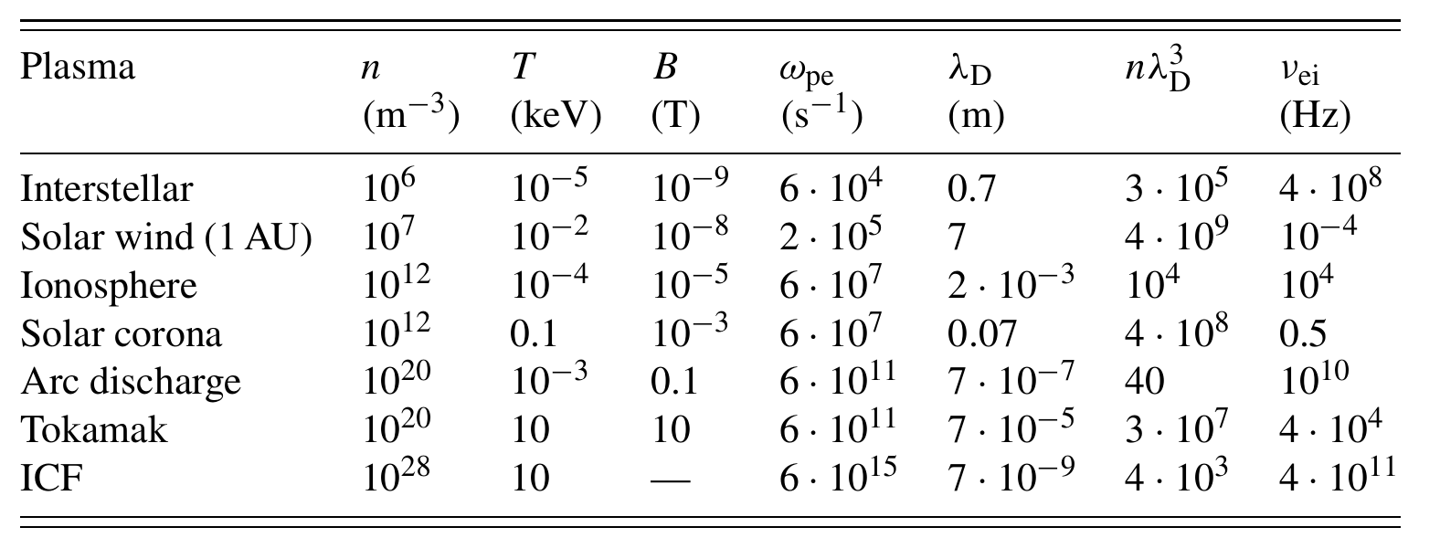
ICF = Inertial Confinement Fusion
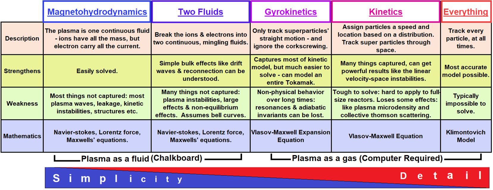
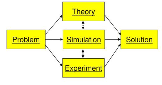
5.1 The role of simulations in science
5.2 Hierarchy of plasma physics models
Kinetic description
Microscopic properties, it uses the velocity distribution function \(f(\vec{x}, \vec{v}, t)\).
Fluid description
Uses a few macroscopic quantities, averages of the distribution function (mean velocity \(v(\vec{x},t)\), pressure/temperature). Valid for exact or near thermodynamic equilibrium.
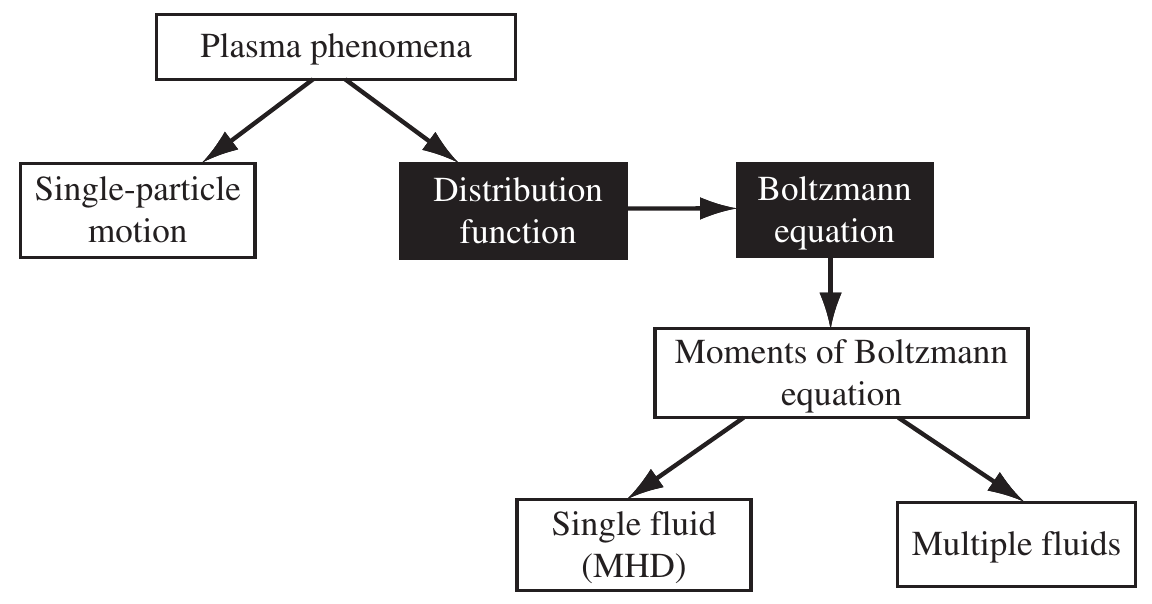
Hierarchy of plasma physics models
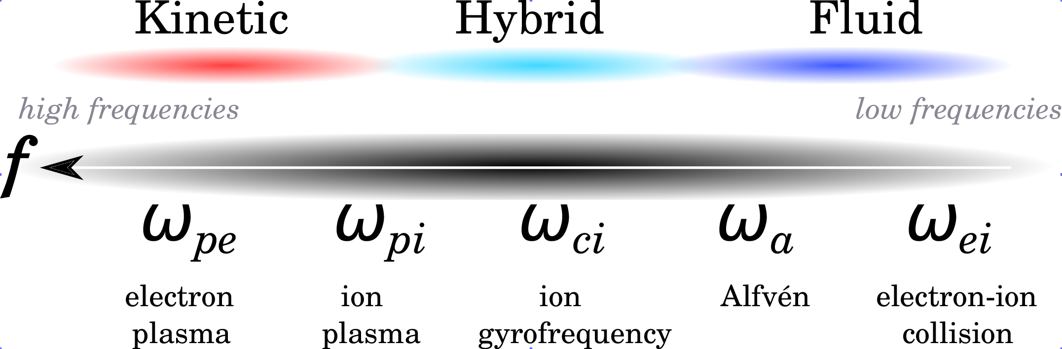
5.3 Validity of plasma models

Range of validity of different plasma codes based on typical magnetospheric parameters: \(n=50cm^{-3}\), \(B=50 nT\), \(T_e=T_i=100 eV\) (Winske and Omidi 1996).
5.4 Validity of plasma models
 Validity range of different plasma codes for a weakly collisional plasma [Credits: space.aalto.fi.]
5.7 Advantages and drawbacks of plasma simulations codes