Lecture 4: Test particles – lecture + hands-on
November 14, 2024
1.5 4th-order Runge Kutta
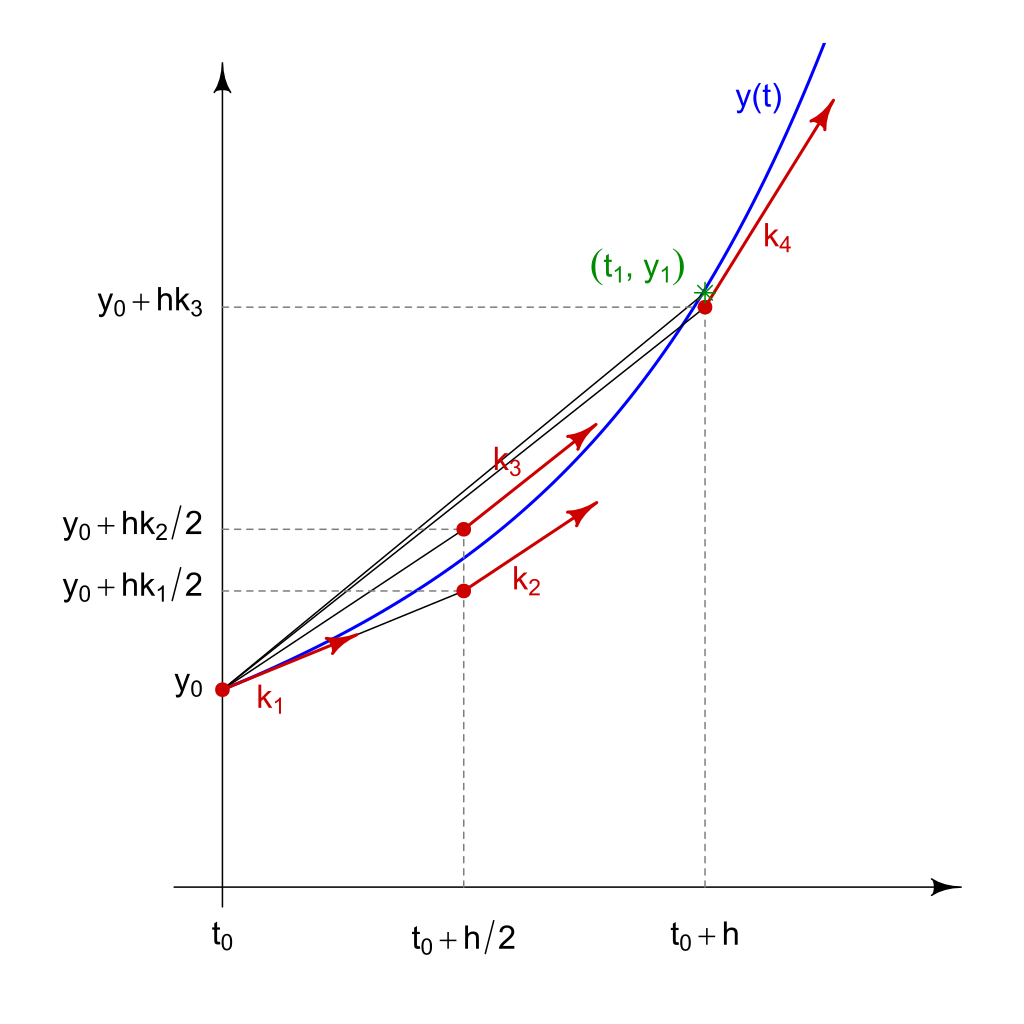
Slopes used for the Runge-Kutta method; \(h = \Delta t\)
1.6 4th-order Runge Kutta
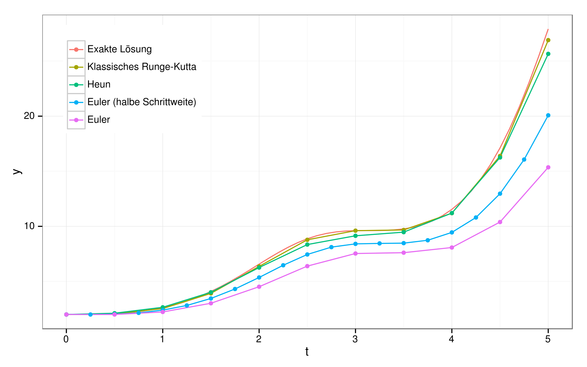
Comparison of Runge-Kutta with other methods for the solution of the ODE: \(y'=sin^2(t)*y\)
1.13 Boris algorithm
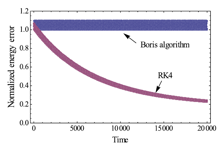
Comparison of energies of a charged particle moving in a given B-field, with its trajectory calculated using the RK4 and Boris algorithms (Qin et al. (2013))
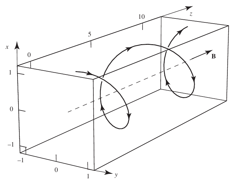
2.6 Particle motion in magnetic fields (helical motion)
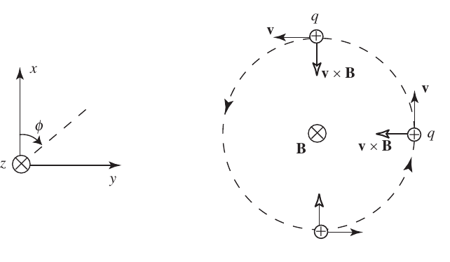
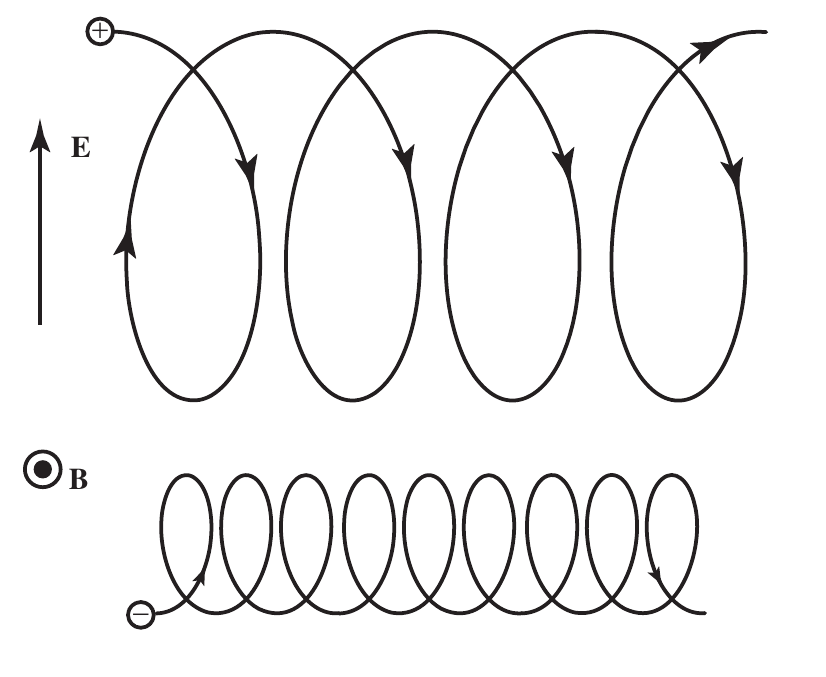
2.9 \(\vec{E}\times\vec{B}\) drift
- The average of \(\vec{v}\) over one gyroperiod is: \[ \langle \vec{v} \rangle = \hat{z} v_{\parallel} + \vec{v}_E \] so \(\vec{v}_E\) is the average perpendicular velocity.
- This drift arises from the difference in the local gyroradius between top/bottom.
- The \(\vec{E}\times\vec{B}\) drift is independent on \(q\), \(m\) and \(v_{\perp}\).
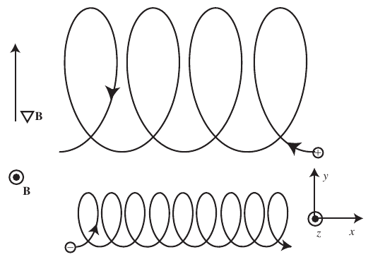
2.10 Gradient B drift
- Let us assume a magnetic field with intensity varying in the perpendicular direction to the B-vector \(\vec{B}(y)=\hat{z}B_z(y)\).
- This drift also arises from a force perpendicular to the magnetic field. Generalizing the expression for the \(\vec{E}\times\vec{B}\) force: \[ \vec{v}_F=\frac{\left( \frac{\vec{F}_{\perp}}{q} \right) \times\vec{B}}{B^2} \]
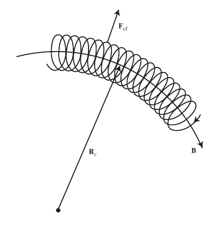
2.12 Curvature B drift
- In a curved magnetic field line, particles experience a centrifugal force perpendicular to the B-field \[
\vec{F}_{cf}=mv_{\parallel}^2\frac{\vec{R}_c}{R_c^2}
\] which causes a drift perpendicular to both vectors.
![]()
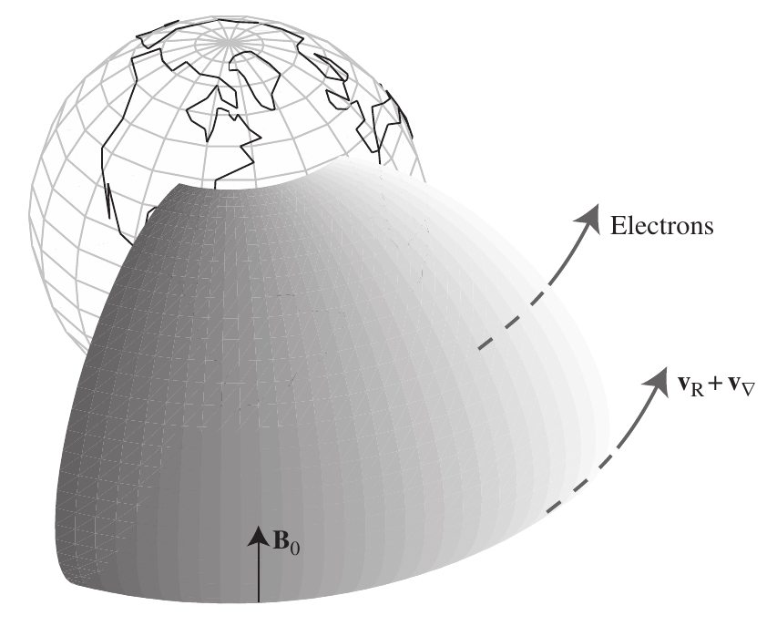
2.14 Curvature B drift
- Longitudinal drift of radiation belt electrons (and associated ring current because of opposite ion/electron drift)
![]()
2.15 Adiabatic invariance of the magnetic moment
- Magnetic moment \(\mu=\frac{mv_{\perp}^2}{2B}\) tends to be conserved as long as (spatial or temporal) changes in B are small over a gyroradius or gyroperiod.
- The particle’s perpendicular energy increases while its parallel energy decreases as it moves toward regions of stronger B, until it eventually \(v_{\parallel}=0\) and it bounces back (magnetic mirror/bottle).

2.16 Particle trajectories in the Earth’s magnetosphere
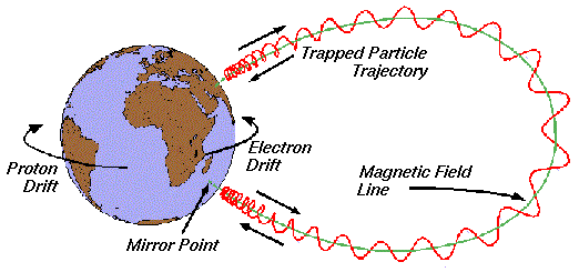
Credits: Spenvis (ESA’s SPace ENVironment Information System) Models description
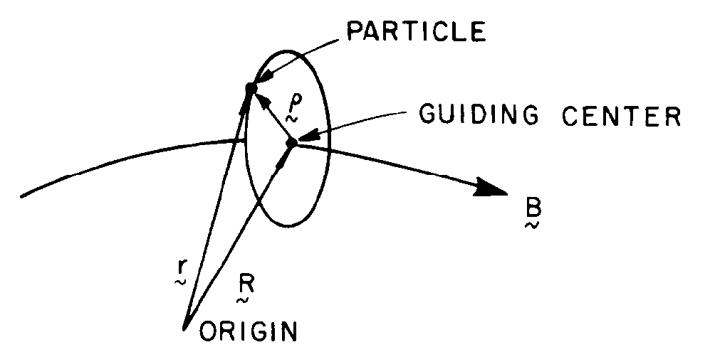
2.18 Guiding center approximation
Valid when the gyroradius (\(\rho= \frac{mv}{qB}\)) and gyroperiod (\(\propto \frac{1}{\Omega} = \frac{m}{qB}\)) are much smaller than the length scale of transverse gradients and characteristic oscillation periods of the background EM fields.
The motion of a charged particle is described in terms of variables representing the gyration around B-field lines and the motion of its guiding center.
For the solar corona, typical gyroradii are \(10^{-3} m\) for electrons and \(10^{-2} m\) for protons, much smaller than typical characteristic lengths scales.