Lecture 5: Particle-in-cell – lecture

Jan Benáček

Institute for Physics and Astronomy, University of Potsdam

November 21, 2024

1 Lecture overview

Table of Contents 1/2

17.10. Introduction + numerical methods summary
24.10. Numerical methods of differential equations — lecture + hands-on
31.10. State holiday
07.11. Test particle approach — lecture
14.11. Test particle approach — lecture + hands-on
21.11. PIC method — lecture
28.11. PIC method — hands-on

Table of Contents 2/2

05.12. Fluid and MHD — lecture
12.12. Fluid and MHD — hands-on
19.12. Canceled
09.01. Radiative transfer — lecture + hands-on
16.01. HPC computing — lecture + hands-on
23.01. Advanced — Smooth particle hydrodynamics method — lecture
30.01. Advanced — Hybrid, Gyrokinetics — lecture
06.02. Advanced — Vlasov and Linear Vlasov dispersion solvers — lecture

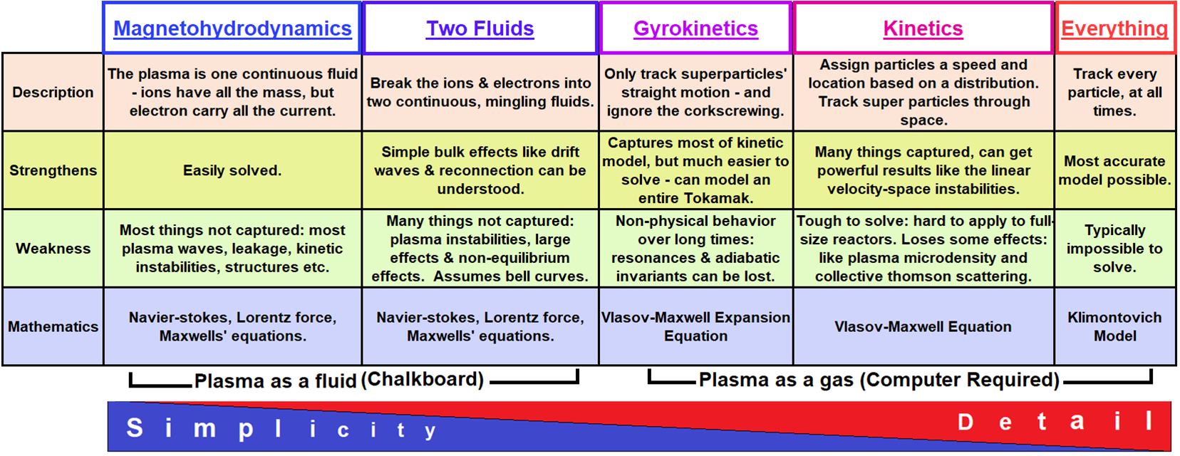
1.1 Fluid vs Kinetic plasma models

Range of validity of different plasma codes based on typical magnetospheric parameters: $n=50cm^{-3}$, $B=50 nT$, $T_e=T_i=100 eV$ (Winske and Omidi (1996)).

1.2 Hierarchy of plasma physics models

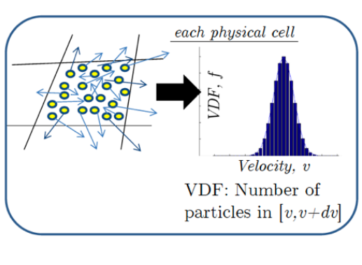
Kinetic description:

Microscopic properties, it uses the velocity distribution function $f$.

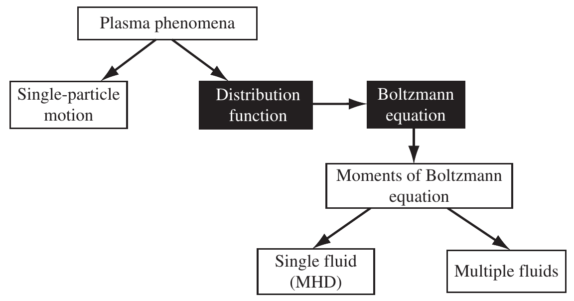
Hierarchy of plasma physics models (Inan and Golkowsky (2011)).

1.3 Vlasov equation 1

Note that here $\vec{E}$ and $\vec{B}$ are long-range averaged (in space and time) macroscopic fields from all the plasma particles and external sources (but not microscopic fields due to binary collisions – collisionless approach).

Vlasov equation

\[ \frac{Df_{\alpha}(\vec{x},\vec{v},t)}{Dt}=\left[\frac{\partial}{\partial t} + \vec{v}\cdot\frac{\partial}{\partial \vec{x}}+\frac{q_{\alpha}}{m_{\alpha}}\left(\vec{E}(\vec{x},t)+\vec{v}\times\vec{B}(\vec{x},t)\right)\cdot\frac{\partial}{\partial \vec{v}}\right]f_{\alpha}(\vec{x},\vec{v},t)=0 \qquad(1)\]

Consequence: $f$ can be expressed in terms of the constants of motion (e.g: energy).
This equation also known as Boltzman equation, if on the RHS term $\left( \frac{\partial f }{\partial t} \right)_\mathrm{coll}$ is zero.

1.4 Vlasov equation 2 — Liouville’s theorem

The theorem valid only for colissionless plasmas
Liouville’s theorem: in absence of collisions, $f$ is invariant along the trajectories in the 6D phase space.

$\rightarrow$ Time-conservation of $f(\vec{x},\vec{v},t) d\vec{x} d\vec{v}$ in the phase space:
Convective derivative: \[ \frac{D}{Dt} = \frac{\partial}{\partial t} + \vec{v}\cdot \frac{\partial}{\partial\vec{x}} + \vec{a}\cdot \frac{\partial}{\partial\vec{v}} = 0 \]
Acceleration due to Lorentz force: $\vec{a}=\left( \frac{q}{m} \right) \left(\vec{E}+\vec{v}\times\vec{B}\right)$.

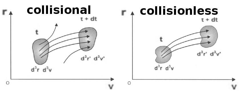
Collisions and conservation of phase space (Bittencourt (2004)).

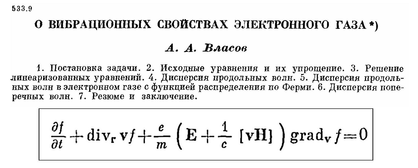
1.5 Vlasov equation

Vlasov, A. A. (1938). The vibrational properties of an electron gas. Zhurnal Eksperimental’noi i Teoreticheskoi Fiziki, 8, 291.

Left: Sampling via Vlasov methods. Right: Sampling via PiC methods (Pukhov (2016)).

1.6 Fully-kinetic/Vlasov description

Full equations of motion

\[ \nabla\cdot\vec{E}(\vec{x},t)=\frac{\rho(\vec{x},t)}{\epsilon_0}\\ \nabla\cdot\vec{B}(\vec{x},t)=0\\ \nabla\times\vec{E}(\vec{x},t)=-\frac{\partial \vec{B}(\vec{x},t)}{\partial t}\\ \nabla\times\vec{B}(\vec{x},t)=\mu_0\vec{J}(\vec{x},t)+\mu_0\epsilon_0\frac{\partial \vec{E}(\vec{x},t)}{\partial t} \]

\[ \frac{dv_i}{dt}=\frac{q}{m}\left[\vec{E}(\vec{x}_i,t) + \vec{v}\times\vec{B}(\vec{x}_i,t) \right] \]

\[ \rho(\vec{x},t)=\sum\limits_{\alpha} q_{\alpha}\int\limits dv^3\,\sum_i\delta(\vec{x}-\vec{x_i})\delta(\vec{v}-\vec{v_i})\\ \vec{J}(\vec{x},t)=\sum\limits_{\alpha} q_{\alpha}\int dv^3\,\vec{v}\sum_i\delta(\vec{x}-\vec{x_i})\delta(\vec{v}-\vec{v_i}) \]

2 The PIC method

2.1 The PIC method

2.2 History

First electrostatic (solving Poisson’s equation) PIC codes (with a grid and finite-sized particles) originated at Stanford University in 1963 (Buneman & Hockney)
Improved methods and the basic theory were developed in the late 60’s and early 70’s, including electromagnetic codes (Birdsall, Morse & Nielson, Boris, etc).
The first large-scale simulations were done at Los Alamos for controlled thermonuclear fusion research programs
Standard books: C. K. Birdsall and Langdon (1991) and Büchner (2023).
Recent review paper: Nishikawa et al. (2021) and Pohl, Hoshino, and Niemiec (2020).
For a history, see Charles K. Birdsall (1999).

2.3 Validity of the fully-kinetic model

Range of validity of different plasma codes based on typical magnetospheric parameters: $n=50cm^{-3}$, $B=50 nT$, $T_e=T_i=100 eV$ (Winske and Omidi (1996)).

2.4 Validity of the fully-kinetic model

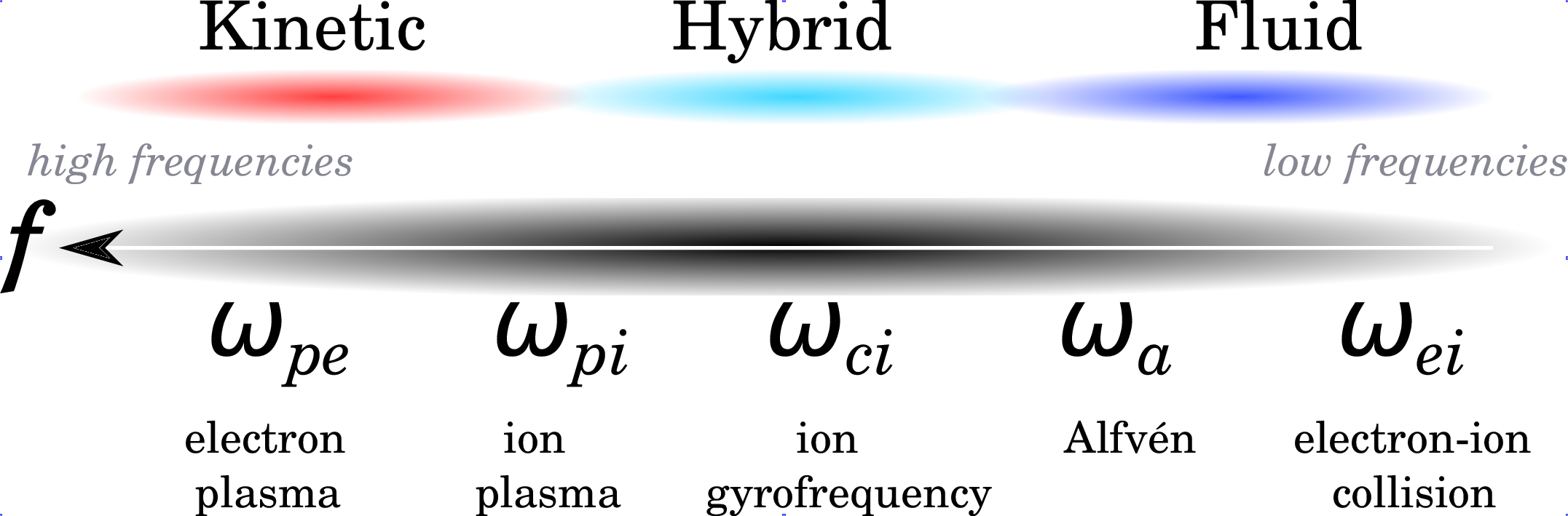
Validity range of different plasma codes [Credits: space.aalto.fi.]

2.5 Fluid vs Kinetic plasma models

$Kn$ is the Knudsen number, which indicates how collisional a plasma is. A collisionless plasma has $K_n\gg1$.

2.6 Fully kinetic approach: PIC codes

Particle-in-Cell (PiC) codes

Electro-magnetic fields allocated on a discrete grid (cell).
Interaction between particles through the electromagnetic fields on the mesh ($\sim N\log(N)$ in Particle-Mesh vs $N^2$ in Particle-Particle)

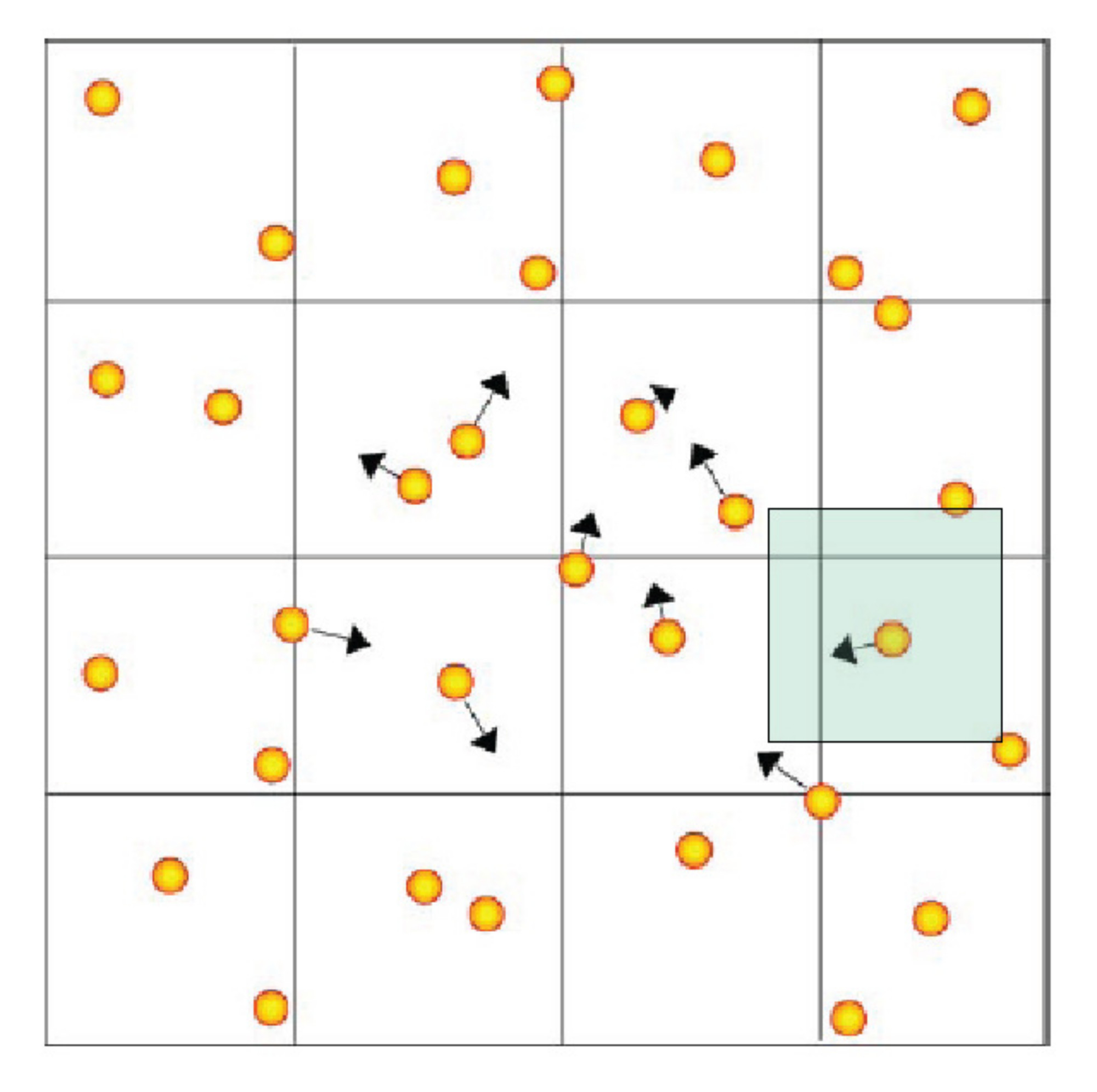
2.7 Sampling of phase space in PIC codes

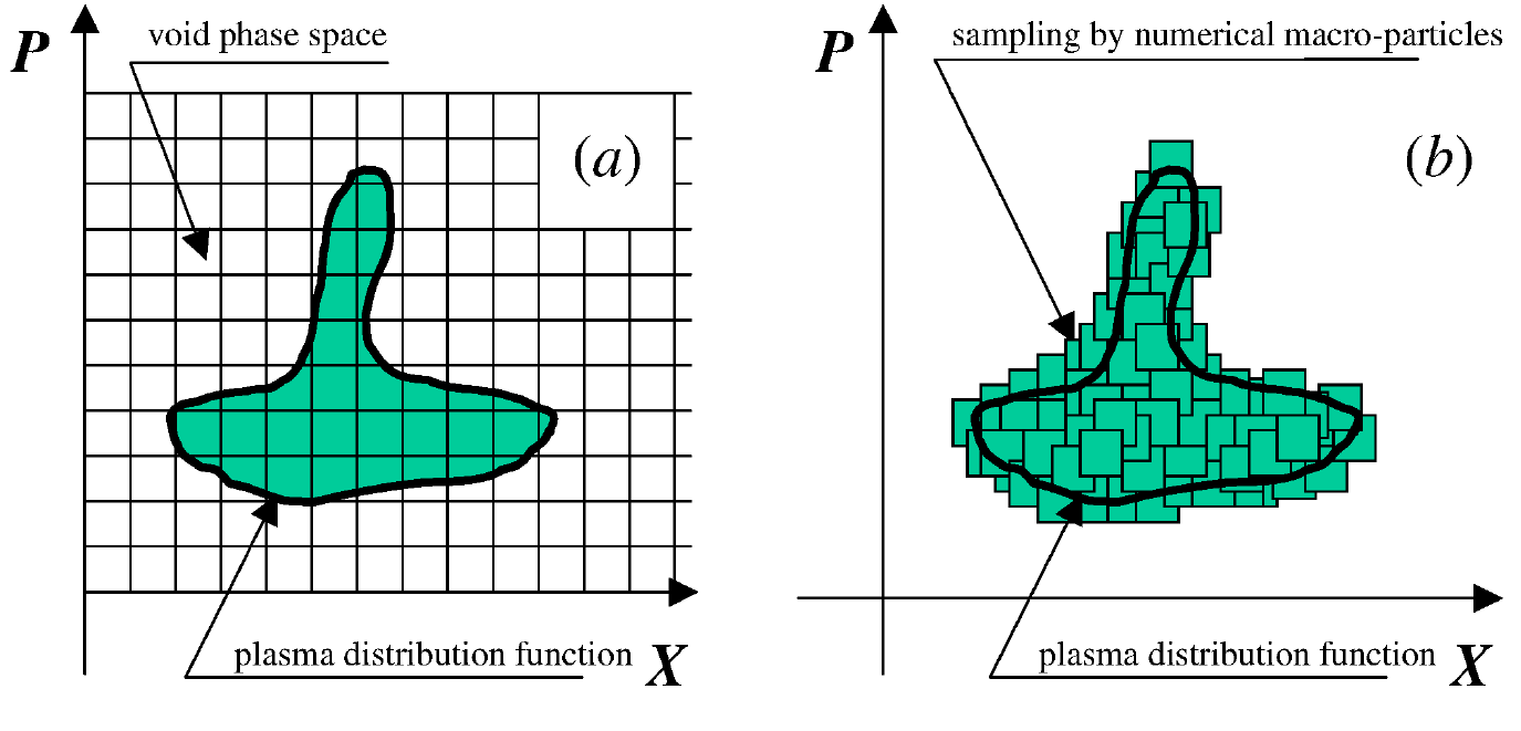
Left: Sampling via Vlasov methods (Eulerian). Right: Sampling via PiC methods (Lagrangian)~(Pukhov 2016).

2.8 Super/Macro-particles

It is not practical to simulate all the particles in a real plasma (e.g.: $10^{16}\;km^{-3}$ in space).
Each simulation particle in a plasma represents many particles, the ratio is (sometimes) called macrofactor $M$. \[ \frac{N_{\rm phys}}{N_{\rm numerical}} = M \] (e.g.: $M=10^3$-$10^{11}$) Simulations can handle around $10^9$ macro-particles.
Charge/mass ratio and charge density remains invariant $\rightarrow$ also $\omega_{pe}$.
The forces (and collisions) between macroparticles are much larger than between real particles.
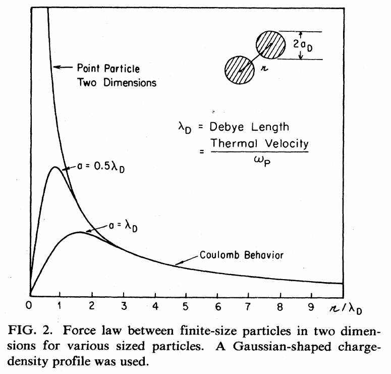
The size of a macroparticle is extended (not point-like).

Macroparticle and its charge density

2.9 Super/Macro-particles

Short/large range force responsible for collisions/collective effects.
Coarse graining effect: close-range collisions are smeared out (reduced) by using finite size particles ($\gtrsim\lambda_{De}$)
Compensation effect on collisions: $\frac{\nu}{\omega_{pe}} \sim \frac{1}{ n \lambda_{De}^3 }$ (regime of interest is $n \lambda_{De}^3 \gg 1$ ), where $\nu$: collision frequency.

Dawson (1983).

2.10 Coarse graining of the distribution function

The physical VDF is represented by: \[ f(\vec{x},\vec{v},t) = \sum_p M_pS_x(\vec{x} - \vec{x}_p)S_v(\vec{v} - \vec{v}_p(t)) =\sum_ pf_p(\vec{x},\vec{v},t) \] with the macroparticle VDF $f_p$: \[ f_p(\vec{x},\vec{v},t) = M_pS_x(\vec{x} - \vec{x}_p(t))S_v(\vec{v} - \vec{v}_p(t)), \qquad(2)\]
$S_x$ and $S_v$ are the shape functions in $\vec{x}$ and $\vec{v}$ space, respectively.
$S_v$ is just a product of Dirac’s deltas: $S_v=\delta(\vec{v} - \vec{v}_p(t))$
There are many choices for the shape function $S_x$. Usually b-splines are chosen.
Sometimes a weighting function is used, related to $S_x$ by: \[ W(\vec{x}_g - \vec{x}_p) =\int_{\vec{x}_g - \vec{\Delta x}/2}^{\vec{x}_g + \vec{\Delta x}/2} S(\vec{x}'-\vec{x}_p) d^3\vec{x}'. \qquad(3)\] where $\vec{x}_g$ represents a cell vertex.

2.11 Typical shape functions

With $\xi= \frac{ |x-x_i|}{\Delta x}$

NGP: Nearest Grid point: \[ W(\xi)=\begin{cases} 1 & \text{ if $\xi<1/2$},\\ 0 & \text{otherwise.} \end{cases} \]
CIC: Cloud in Cell. \[ W(\xi)=\begin{cases} 1 - \xi & \text{ if $\xi<1$,}\\ 0 & \text{otherwise}. \end{cases} \]
TSC: Triangular Shaped Cloud \[ W(\xi)=\begin{cases} \frac{3}{4} - \xi^2 & \text{ if $\xi<1/2$,}\\ \frac{1}{2}\left(\frac{3}{2} - \xi\right)^2 & \text{ if $1/2<\xi<3/2$,}\\ 0 & \text{otherwise.} \end{cases} \]

2.12 Typical shape functions

Higher order shape functions reduce numerical noise/collisions/heating.

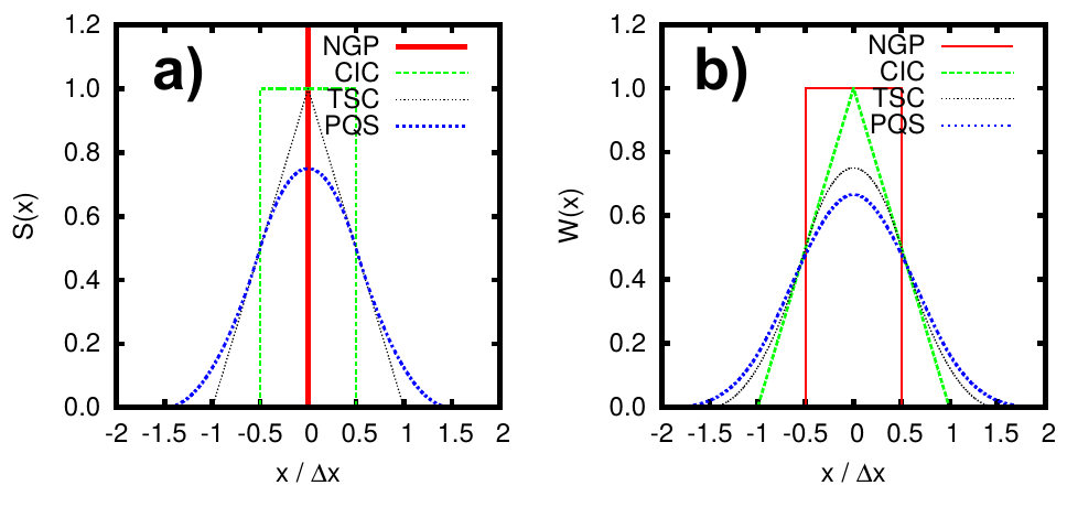
Left: $S(x)$. Right $W(x)$. Both in 1D.

2.13 Typical shape functions

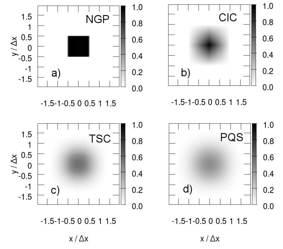
$W(x)W(y)$ functions in 2D.

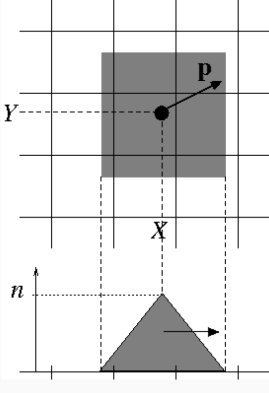
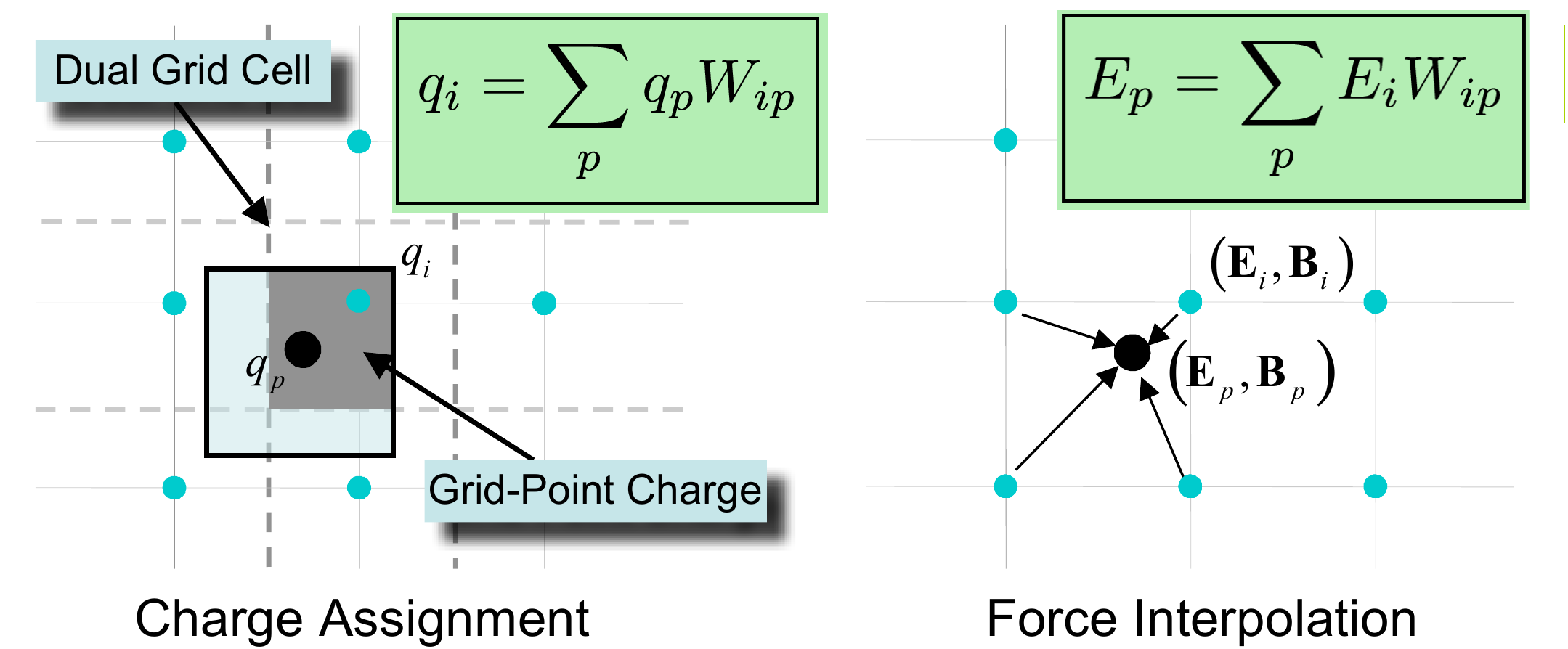
2.14 Weighting and interpolation

Shape function $S(x)$ assigns $\rho$ and $J$ to grid points, and (inversely) interpolates E-M fields to the particles position.

2.15 Discrete Vlasov equation

Velocity moment of order one $\int \vec{v} d^3\vec{x} d^3\vec{v}$ (Vlasov eq.): \[ \frac{d\vec{v}_p}{dt}=\frac{q_p}{m_p}\left[\vec{E}_p(\vec{x},t)+\vec{v}_p\times\vec{B}_p(\vec{x},t)\right] \qquad(4)\] i.e.: formally equivalent to the Lorentz force, but with the EM fields defined (sampled) only at the grid points: \[ \vec{E}_p=\vec{E}(\vec{x}_p) = \int \vec{E}(\vec{x})S(\vec{x} -\vec{x}_p)=\sum_{\vec{x}_c}\vec{E}(\vec{x}_c)W(\vec{x}_c - \vec{x}_p)\\ \vec{B}_p=\vec{B}(\vec{x}_p) = \int \vec{B}(\vec{x})S(\vec{x} -\vec{x}_p)=\sum_{\vec{x}_c}\vec{B}(\vec{x}_c)W(\vec{x}_c - \vec{x}_p) \qquad(5)\]
$q_p$ and $m_p$ corresponds to the charge and mass of each macroparticle (not the physical particle)
The sum runs over all the cell vertices (subscript $\vec{c}$) at the boundaries of each cell volume

2.16 A typical PIC loop

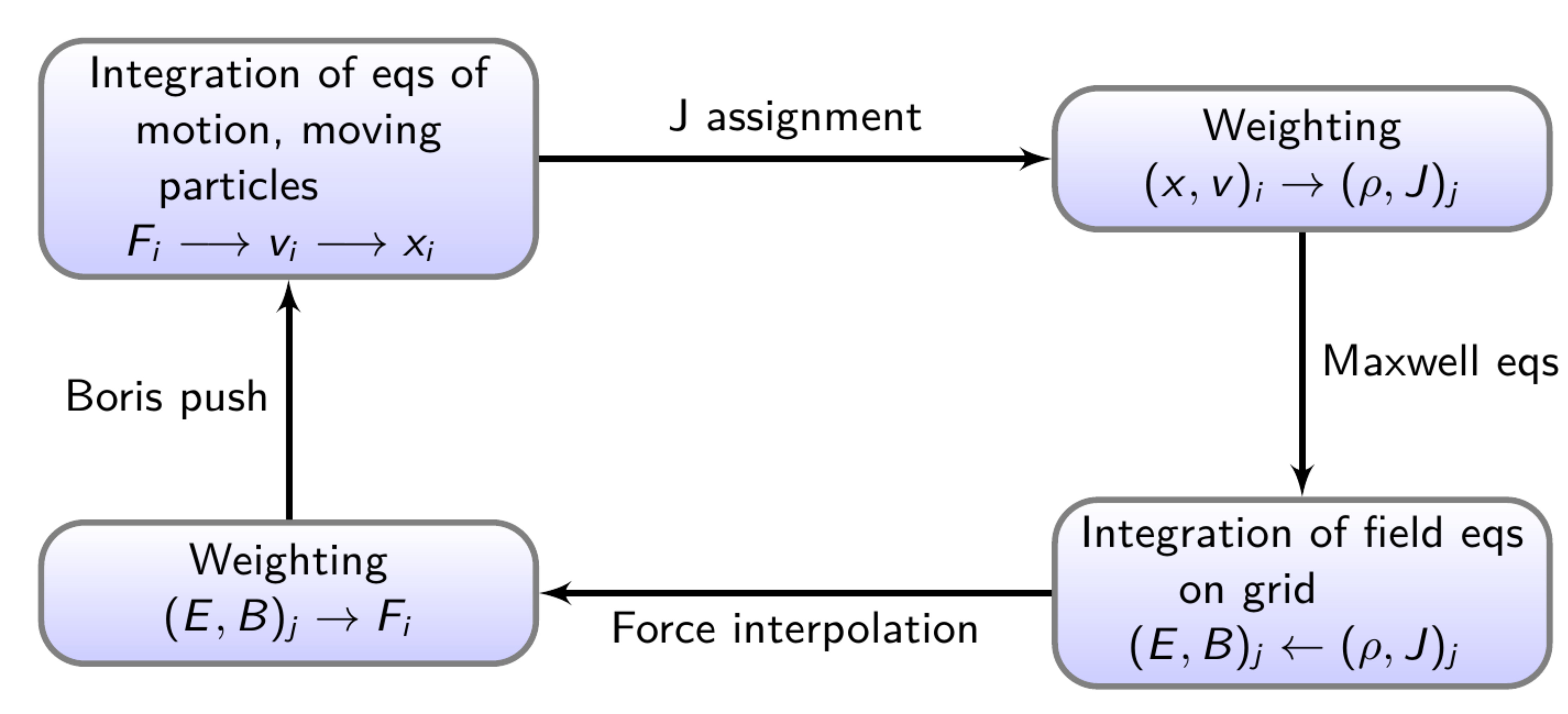
PIC loop.

3 Electrostatic codes

3.1 Electrostatic plasma approximation

3.2 Electrostatic plasma approximation

There are different types of plasma models where a PIC code can be used: electrostatic, electromagnetic, Darwin, etc.
Electrostatic plasma approximation: for high frequency phenomena and small length scales.
Charge separation can occur.
Currents are assumed small ($\vec{J}\approx 0$), so self-magnetic fields are small: $\nabla\times\vec{B}=0$ and $\nabla\times\vec{E}=0$
It is convenient then to introduce the electrostatic potential $\phi$. \[ \vec{E}=-\nabla\phi \]

3.3 Electrostatic plasma approximation

Electrostatic (ES) plasma model

\[ \nabla^2\phi=-\frac{\rho}{\epsilon_0}\\ \nabla\cdot\vec{B}=0 \]

\[ \left[\frac{\partial}{\partial t} + \vec{v}\cdot\frac{\partial}{\partial \vec{x}}+\frac{q_{\alpha}}{m_{\alpha}}\left(\vec{E}+\vec{v}\times\vec{B}_0\right)\cdot\frac{\partial}{\partial \vec{v}}\right]f_{\alpha}=0\\ \rho=\sum\limits_{\alpha} q_{\alpha}\int\limits dv^3\,f_{\alpha} \]

Note that Poisson’s equation is an elliptic equation with no real characteristics $\Rightarrow$ the nature of the equations is different from the hyperbolic fully-kinetic plasma model.

3.4 Electrostatic codes

3.5 Particle charge and force weighting

In electrostatic PIC codes, it is necessary to calculate $\rho$ at the grid points, as well as $\vec{E}$ at the particle position.
Example in 1D, using CIC shape function:

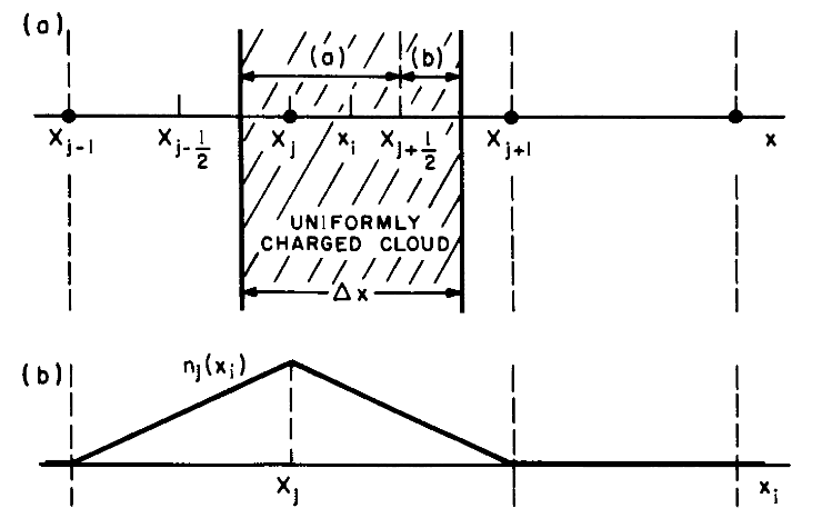
First order particle weighting (C. K. Birdsall and Langdon (1991)).

3.6 Force weighting

The same weighting scheme as for the particles is used for the forces: \[ \vec{E}=\sum_i E_i S(\vec{x}_i - \vec{x}) \]
The consequence is that the self-force for the particle located at x vanishes: \[ F_{self}= e\sum_i E_i S(x_i - x)=0 \]
If we also assume a symmetric $E_i=\sum_k g_{ik}\rho_k$ with $g_{ik}=-g_{ki}$, the two-particle interaction force becomes \[ F_{12}= e_1E_2(x_1)=e_1\sum_i E_{2,i}S(x_i-x_1)=-e_2E_1(x_2)=-F_{21} \]

3.7 Momentum conservation

This kind of PIC schemes conserves momentum \[ \frac{dP}{dt}=F=\sum_{p=1}^N e_p\left(\vec{E}(\vec{x}_p) + \vec{V}_p\times\vec{B}(\vec{x}_p)\right)=\Delta x^3\sum_i(\rho_i\vec{E}_i^{ext} + \vec{J}_i\times\vec{B}_i^{ext}) \]
But those schemes do not conserve energy…
There are energy-conserving PIC schemes, but they do not conserve momentum…

3.8 Integration of fields equations

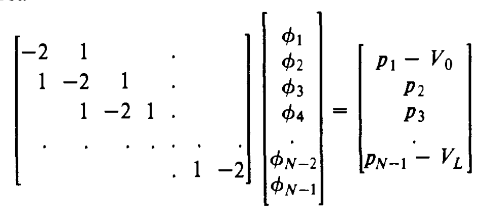
Discretized form of the Poisson’s equation: \[ \frac{\phi_{j-1} - 2\phi_j + \phi_{j+1}}{\Delta x^2} = -\frac{\rho_j}{\epsilon_0} \] which can be written in matrix form: \[ \hat{A}\phi_j = -\frac{\Delta x^2}{\epsilon_0}\rho_j \]
This matrix equation can be solved by standard methods. It is usually in tri-diagonal form, boundary conditions should be considered.

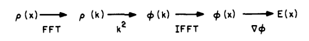
3.9 Integration of fields equations: Fourier methods

For periodic boundaries conditions, Fourier methods are preferred
They are based on the Fast Fourier Transform (FFT) since the 60s.
Assuming a dependence for $\rho(\vec{k}),\phi(\vec{k})\propto \exp(-i\vec{k}\cdot\vec{x})$: \[ \phi(k)=\frac{\rho(k)}{\epsilon_0 k^2} \qquad(6)\]
Then, we take the inverse Fourier transform to obtain $\phi(\vec{k})$

3.10 Integration of fields equations: Fourier methods

Discrete Fourier transform (for the generic function $F(x)$) \[ F(k)=\Delta x\sum_{j=0}^{N-1}F(X_j)\exp(-ikX_j) \]
Inverse Fourier transform (for $k=n2\pi/L$) \[ F(X_j)=\frac{1}{L} \sum_{j=-N/2}^{N/2-1}F(k)\exp(ikX_j) \]

3.11 Integration of the equations of motion

Conventional wisdom: Leapfrog method, because it achieves a good balance between accuracy, stability and efficiency.
The finite difference equations are: \[ m\frac{\vec{v}_i^{n+1/2} -\vec{v}_i^{n-1/2}}{\Delta t} = qE_i^n\\ \frac{x_i^{n+1} - x_i^n}{\Delta t}= \vec{v}_i^{n+1/2} \]

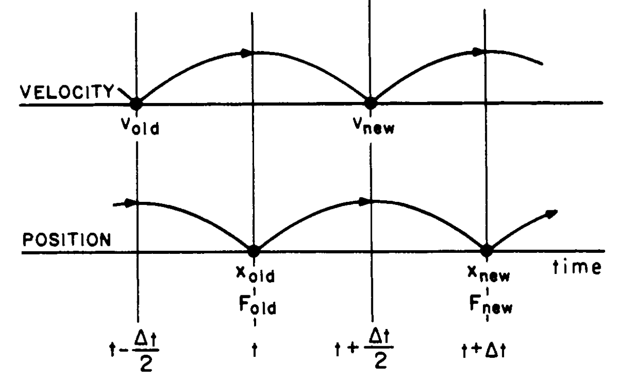
Leapfrog scheme (Charles K. Birdsall (1999)).

3.12 Integration of the equations of motion

For particles in harmonic motion. \[ \frac{d^2x}{dt^2}= -\omega_0^2 x \]
The finite difference becomes \[ \sin\left(\frac{\omega \Delta t}{2}\right)= \pm\frac{\omega_0 \Delta t}{2} \]
Leapfrog is stable if $\omega_{0}\Delta t \leq 2$.
The relevant frequency is $\omega_0=\omega_{pe}$, but accuracy for plasma waves requires $\omega_{pe}\Delta t< 0.2$.

3.13 Integration of the equations of motion

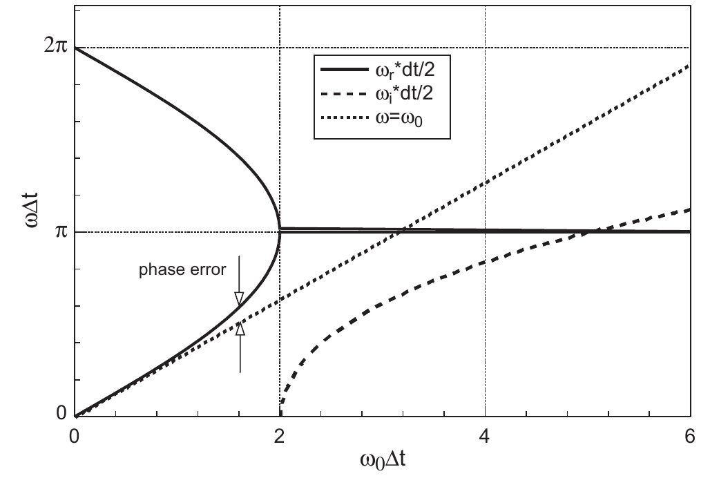
Leapfrog scheme: Real frequency $\omega_r$ and numerical growth rate $\omega_i$. Phase error is the difference with the exact frequency $\omega_0$ (Verboncoeur (2005)).

3.14 Integration of the equations of motion

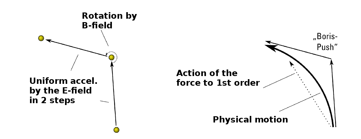
When magnetic fields are present, the Boris algorithm is used.
For 1D case, along $x$, $\vec{B}=B_0\hat{z}$ and $\vec{E}=E\hat{x}$.
3-stage particle motion: half-acceleration, rotation by B, and half-acceleration.

Geometry for the Boris algorithm (C. K. Birdsall and Langdon (1991)).

3.15 Integration of the equations of motion

Half-acceleration \[ v_x(t') = v_x\left(t-\frac{\Delta t}{2} \right) + \frac{q}{m}E_x(t) \left(\frac{\Delta t}{2}\right)\\ v_y(t') = v_y\left(t-\frac{\Delta t}{2} \right) \]
Rotation by $\Delta \theta= -\Omega_{c}\Delta t$ ($\omega_c = qB / m$ is the cyclotron frequency) \[ \begin{pmatrix} v_x(t'') \\ v_y(t'') \end{pmatrix} = \begin{pmatrix} \cos(\Omega_c \Delta t) & \sin(\Omega_c \Delta t) \\ -\sin(\Omega_c \Delta t) & \cos(\Omega_c \Delta t) \\ \end{pmatrix} \begin{pmatrix} v_x(t') \\ v_y(t') \end{pmatrix} \]
Half-acceleration \[ v_x\left(t + \frac{\Delta t}{2} \right) = v_x(t'') + \frac{q}{m} E_x(t) \left(\frac{\Delta t}{2}\right)\\ v_y\left(t + \frac{\Delta t}{2} \right) = v_y(t'') \]

4 Electromagnetic PIC algorithm

4.1 Electromagnetic PIC algorithm

4.2 Maxwell solver

4.3 Maxwell equations: FDTD method

Faraday’s and Ampere’s laws are hyperbolic equations for the evolution of $\vec{B}$ and $\vec{E}$, respectively.
Most of the fully-kinetic PIC codes solve those equations via the Finite Difference Time-Domain (FDTD) method: \[ \vec{B}^{i+1/2} = \vec{B}^{i-1/2} - \Delta t \left(\nabla\times\vec{E}^i \right)\\ \vec{E}^{i+1} = \vec{E}^{i} + \Delta t \left(\nabla\times\vec{B}^{i+1/2} \right) - \mu_0 \Delta t \vec{J}^{i+1/2} \] Alternative: spectral Fourier methods
FDTD methods were developed since the end of the 60s, mainly for military defense applications (radar, EMP, etc)
It is popular because of: no linear algebra, accurate and robust, treats impulsive behaviors naturally, easy to parallelize, etc. (Taflove and Hagness (2005)).

4.4 Yee lattice: fundamentals

Yee (1966) proposed a specific arrangement of the electromagnetic fields on a lattice.
The reasoning behind the arrangement is the calculation of the curl by finite differences, for example: \[ \left(\nabla\times\vec{E}\right)_{x} = \frac{\partial E_z}{\partial y} - \frac{\partial E_y}{\partial z} \approx \frac{E_{z,(i,j+1,k)} - E_{z,(i,j,k)}}{\Delta y} - \frac{E_{y,(i,j,k+1)} - E_{y,(i,j,k)}}{\Delta z} \qquad(7)\]

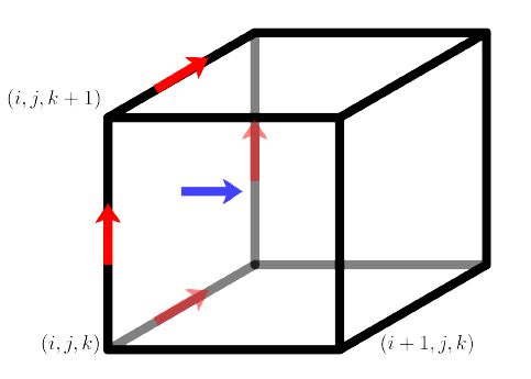
Red: $\vec{E}$ (RHS Equation 7). Blue: Resulting $B_x$

4.5 Yee lattice

Yee lattice: $\vec{E}$, $\vec{B}$, $\vec{J}$ and $\rho$ components.

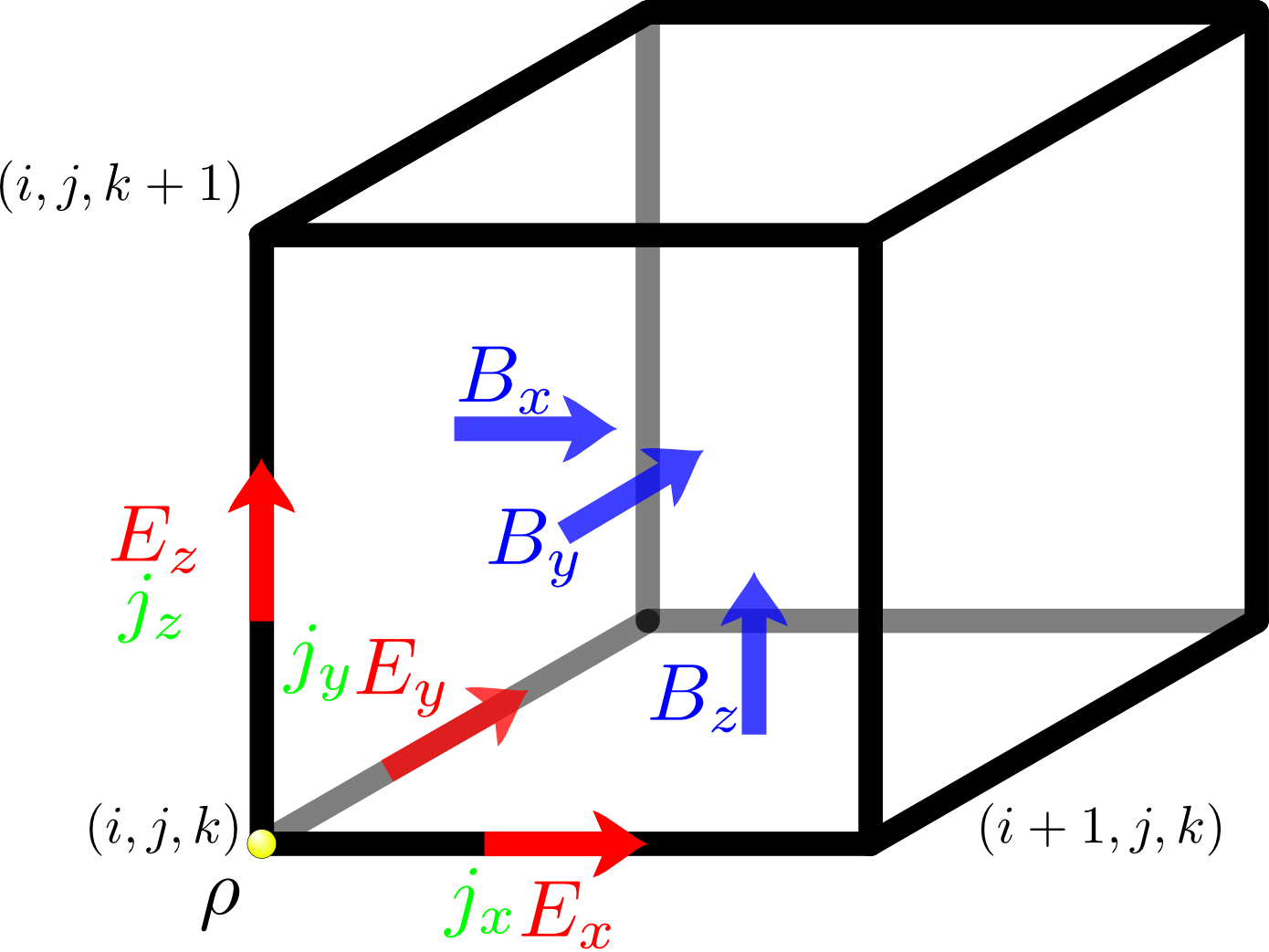
Yee lattice

4.6 Yee lattice: properties

Space derivatives are 2nd-order accurate central differences.
Yee lattice’s $\vec{B}$ components can be associated with magnetic flux linking $\vec{E}$ loops (and viceversa), useful to specify field boundary conditions.
Ihe location of $\vec{E}$ and $\vec{B}$ implicitly enforces the other two divergence Maxwell eqs.
Yee’s algorithm also centers $\vec{E}$ and $\vec{B}$ components in time alternatively, leapfrog arrangement. This algorithm is non-dissipative.

4.7 Yee lattice: stability

As any explicit algorithm for the solution of hyperbolic eqs., the FDTD-Yee algorithm needs to resolve the fastest wave mode in order to be stable. In this case, light waves: \[ \frac{\omega^2}{c^2}=k_x^2+ k_y^2+k_z^2 \qquad(8)\]
By using the discretized form of Ampere’s+Faraday’s equations, and assuming harmonic solutions: \[ \left(\frac{\sin(\omega \Delta t/2)}{c\Delta t}\right)^2 = \left(\frac{\sin(k_x \Delta x/2)}{\Delta x}\right)^2 + \left(\frac{\sin(k_y \Delta y/2)}{\Delta y}\right)^2 + \left(\frac{\sin(k_z \Delta z/2)}{\Delta z}\right)^2 \qquad(9)\]
By imposing real solutions for $\omega$ ($\sin^2(\omega\Delta t/2)\leq 1$), we get the Courant-Friedrichs-Lewy (CFL) condition condition (Courant, Friedrichs, and Lewy (1928)): \[ c\Delta t_c \leq \min\left\{ \Delta x, \frac{\Delta x}{\sqrt{2}},\frac{\Delta x}{\sqrt{3}} \right\} = \frac{\Delta x}{\sqrt{3}}\;\;\text{in 3D}. \qquad(10)\]

4.8 Yee lattice: stability

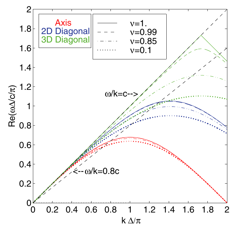
FDTD numerical dispersions relation for light waves: physical, propagation along a grid axis, 2D grid diagonal and 3D grid diagonal.$\Delta t=\nu \Delta_{t,max}= \nu \Delta x \sqrt{3}/c$.

4.9 Current deposition

4.10 Current deposition schemes

Solving equation \[ \frac{\partial \vec{E}}{\partial t} = \epsilon_0 \nabla \times \vec{B} + \epsilon_0 \mu_0 \vec{J}, \qquad \vec{J} = \sum_i q_i \vec{v_i} \]
Note that we only need $\vec{J}$ to solve Maxwell eqs, not $\rho$ ($\nabla \vec{E} = \rho / \epsilon_0$, which was used in electrostatic case).
The direct (naive) current deposition scheme is: \[ \vec{J}(\vec{X}_{i,j,k}) = \sum_n M_n q_{\alpha}\vec{v}_n S(\vec{x}_n - \vec{X}_{i,j,k}) \] where $\vec{X}_{i,j,k}$ is a grid cell coordinate, $\vec{x}_n$ the particles’ coordinates with velocity $v_n$, $M_n$ the macrofactor.
But this method does not satisfy the continuity equation for $\rho$ and $\vec{J}$.
One solution is to correct Poisson’s eq by solving it (previous lecture)
But there are clever (but more complex) way to deposit the current.

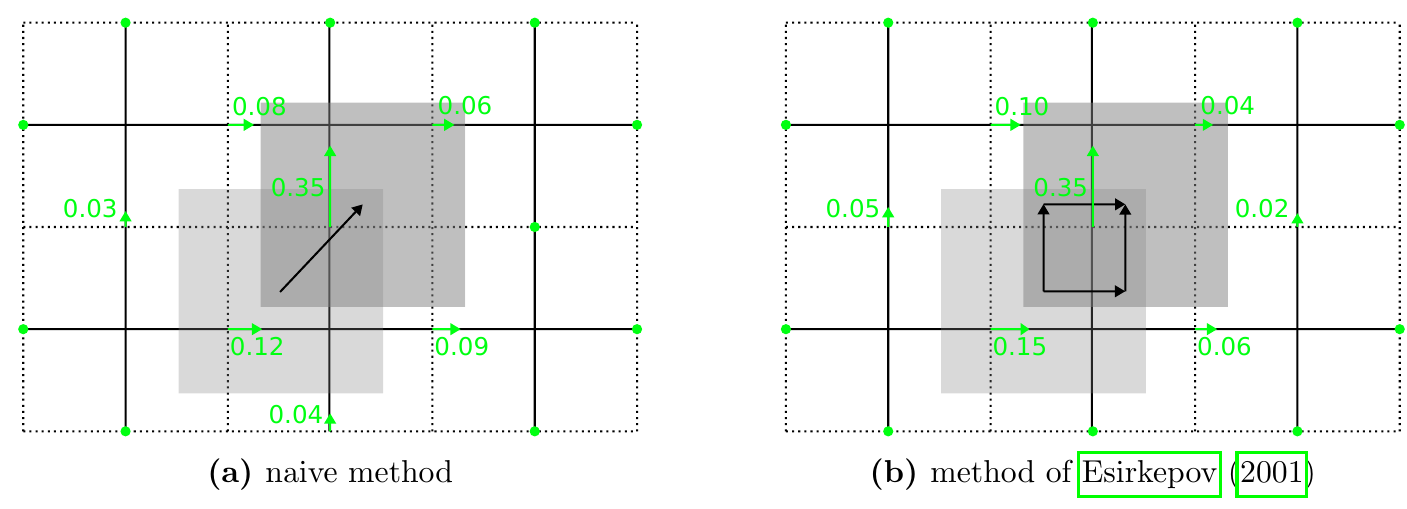
4.11 Current deposition schemes: Esirkepov

Esirkepov (2001) proposed a deposition method based on the displacement of the charges in the cell between timesteps $t$ and $t+1$.
This displacement is obtained from the difference of the shape functions, decomposed into three spatial components.
There are also other charge-conserving current deposition schemes Villasenor and Buneman (1992), Umeda et al. (2003).

4.12 Particle mover

4.13 Boris algorithm

Specifically used to advance particles in plasma simulations (it is the de facto algorithm).
It has very good conservation properties: it , even though it is not symplectic (Qin et al. (2013)).
Discretized (relativistic Lorentz force):

\[ \frac{\vec{x}^{i+1/2} - \vec{x}^{i-1/2}}{\Delta t} = \frac{\vec{v}^{i}}{\gamma^{i}} \\ \frac{\vec{u}^{i+1} - \vec{u}^{i}}{\Delta t} = \frac{q}{m}\left(\vec{E}^{i+1/2} +\vec{v}^{i+1/2} \times\vec{B}^{i+1/2} \right) \] where $\vec{u}=\gamma (c,\vec{v})$ the 4-velocity, $\gamma=\left(1-\left(\frac{v}{c}\right)^2\right)^{-\frac{1}{2}}=\left(1+\left(\frac{u}{c}\right)^2\right)^{-\frac{1}{2}}$ the Lorentz factor.
The idea of the Boris algorithm is to separate the electric and magnetic force in 3 parts: first half of the electric force is determined, then the full magnetic force (rotation), and finally the second half of the electric force.

4.14 Boris push

\[\vec{u}^{-} = \vec{u}^{i} + \frac{q\Delta t}{2m}\vec{E}^{i+1/2} \]
\[ \frac{\vec{u}^{+} - \vec{u}^{-}}{\Delta t} = \frac{q}{m}\left( \vec{v}^{i+1/2}\times\vec{B}^{i+1/2}\right) \]
\[ \vec{u}^{i+1} = \vec{u}^{+} + \frac{q\Delta t}{2m}\vec{E}^{i+1/2} \]

The Boris push.

4.15 Boris push

The phase angle of the rotation (2nd part): \[ \theta = \frac{q\Delta t}{m\gamma^{-}}B^{i+1/2} \]
The rotation is solved in this way: \[ \vec{u}'=\vec{u}^{-} + (\vec{u}^{-}\times\vec{t}) \\ \vec{u}^{+}=\vec{u}^{-} + \frac{2}{1+t^2}(\vec{u}^{'}\times\vec{t}) \] with \[ \vec{t}=\tan \left(\frac{\theta}{2} \right)\vec{b}^{i+1/2} \]
Sometimes the previous equation is approximated as $\vec{t}=(\theta/2)\vec{b}$ (see a comparison in Ripperda et al. (2018), Zenitani and Umeda (2018)).

4.16 Boris algorithm

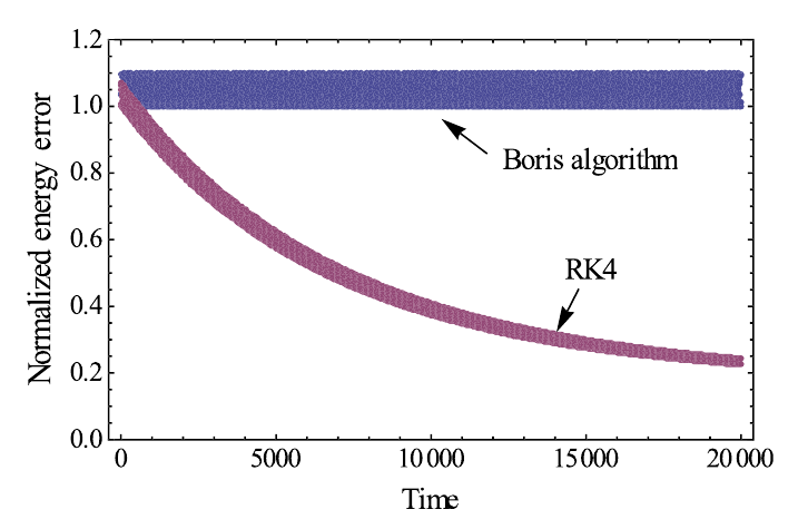
Comparison of energies of a charged particle moving in a given B-field, with its trajectory calculated using the RK4 and Boris algorithms .

4.17 Coupling of particle and field integrations

The field solver gives $\vec{E}^{i+1}$ and $\vec{B}^{i+1/2}$ (and requiring $\vec{J}^{i+1/2}$), while the particle mover $\vec{v}^{i+1}$ and $\vec{x}^{i+1/2}$ (and requiring $\vec{E}^{i+1/2}$ and $\vec{B}^{i+1/2}$)
$\vec{E}^{i+1/2}$ in the particle mover can be obtained by a simple average of $\vec{E}^{i+1}$ and $\vec{E}^{i}$.
$\vec{J}^{i+1/2}$ can be obtained by averaging velocities or shape functions.

5 Conclusions

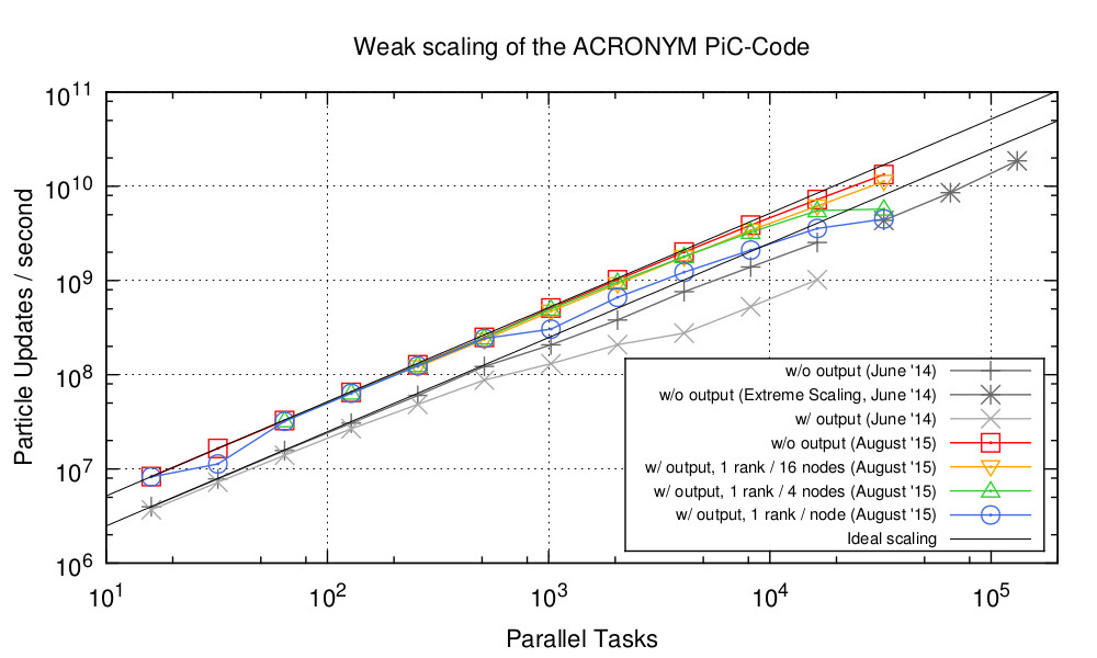
5.1 PIC code ACRONYM

Our fully-kinetic PIC code is called ACRONYM: “Another Code for pushing Relativistic Objects, Now with Yee lattice and Macro particles” http://plasma.nerd2nerd.org
MPI parallelized, good scaling up to $10^5$ cores
Applications: wave-wave interactions in type II and type III solar radio bursts (radio emission), CME driven shocks in the solar wind, resonant wave-particle interactions, current sheet instabilities and magnetic reconnection, kinetic turbulence, particle acceleration, pulsar radio emission.

5.2 Other PIC codes

TRISTAN code: Buneman 1993, Terra Scientific
Spitkovsky/Princeton’s Tristan-MP: https://github.com/ntoles/tristan-mp-pitp
Zeltron: https://ipag.osug.fr/~ceruttbe/Zeltron/index.html
UCLA’s skeleton PIC codes: https://github.com/UCLA-Plasma-Simulation-Group/PIC-skeleton-codes
Los Alamos’s VPIC: https://github.com/lanl/vpic
LLNL/LBNL’ Warp: http://warp.lbl.gov/home
Lapenta/Leuven’s iPic3D: https://github.com/CmPA/iPic3D
UK’s EPOCH: https://gitlab.com/arm-hpc/packages/wikis/packages/EPOCH
HZDR’s PIConGPU: https://github.com/ComputationalRadiationPhysics/picongpu
SMILEI: https://smileipic.github.io/Smilei
ISIRIS: https://osiris-code.github.io

5.3 References

Birdsall, C. K., and A. Bruce Langdon. 1991. Plasma Physics via Computer Simulation. Bristol, England: IOP Publishing. https://www.crcpress.com/Plasma-Physics-via-Computer-Simulation/Birdsall-Langdon/p/book/9780750310253.

Birdsall, Charles K. 1999. “Pioneering in Plasma Simulation.” In Dyn. Syst. Plasmas Gravit. Springer. http://link.springer.com/chapter/10.1007/BFb0105944.

Bittencourt, J. A. 2004. Fundamentals of Plasma Physics. Springer.

Büchner, Jörg. 2023. Space and Astrophysical Plasma Simulation. Methods, Algorithms, and Applications. https://doi.org/10.1007/978-3-031-11870-8.

Courant, R., K. Friedrichs, and H. Lewy. 1928. “Über die partiellen Differenzengleichungen der mathematischen Physik.” Math. Ann. 100 (1): 32–74. https://doi.org/10.1007/BF01448839.

Dawson, John M. 1983. “Particle simulation of plasmas.” Rev. Mod. Phys. 55 (2): 403–47. https://doi.org/10.1103/RevModPhys.55.403.

Esirkepov, T.Zh. 2001. “Exact Charge Conservation Scheme for Particle-in-Cell Simulation with an Arbitrary Form-Factor.” Computer Physics Communications 135 (2): 144–53. https://doi.org/https://doi.org/10.1016/S0010-4655(00)00228-9.

Inan, Umran, and Marek Golkowsky. 2011. Principles of Plasma Physics for Engineers and Scientists. Cambridge University Press.

Nishikawa, Kenichi, Ioana Duţan, Christoph Köhn, and Yosuke Mizuno. 2021. “PIC methods in astrophysics: simulations of relativistic jets and kinetic physics in astrophysical systems.” Living Reviews in Computational Astrophysics 7 (1): 1. https://doi.org/10.1007/s41115-021-00012-0.

Pohl, M., M. Hoshino, and J. Niemiec. 2020. “PIC simulation methods for cosmic radiation and plasma instabilities.” Progress in Particle and Nuclear Physics 111 (March): 103751. https://doi.org/10.1016/j.ppnp.2019.103751.

Pukhov, Alexander. 2016. “Particle-in-Cell Codes for plasma-based particle acceleration.” In Proc. CAS-CERN Accel. Sch., 181. https://doi.org/10.5170/CERN-2016-001.181.

Qin, Hong, Shuangxi Zhang, Jianyuan Xiao, Jian Liu, Yajuan Sun, and William M Tang. 2013. “Why is Boris algorithm so good?” Phys. Plasmas 20 (8): 084503. https://doi.org/10.1063/1.4818428.

Ripperda, B., F. Bacchini, J. Teunissen, C. Xia, O. Porth, L. Sironi, G. Lapenta, and R. Keppens. 2018. “A Comprehensive Comparison of Relativistic Particle Integrators.” Astrophys. J. Suppl. Ser. 235 (1): 21. https://doi.org/10.3847/1538-4365/aab114.

Taflove, A., and S. C. Hagness. 2005. Computational Electrodynamics: The Finite-Difference Time-Domain Method. Artech House Antennas and Propagation Library. Artech House. https://books.google.de/books?id=n2ViQgAACAAJ.

Umeda, Takayuki, Y Omura, T Tominaga, and H Matsumoto. 2003. “A new charge conservation method in electromagnetic particle-in-cell simulations.” Comput. Phys. Commun. 156 (1): 73–85. https://doi.org/10.1016/S0010-4655(03)00437-5.

Verboncoeur, John P. 2005. “Particle simulation of plasmas: review and advances.” Plasma Phys. Control. Fusion 47 (5A): A231–60. https://doi.org/10.1088/0741-3335/47/5A/017.

Villasenor, John, and Oscar Buneman. 1992. “Rigorous charge conservation for local electromagnetic field solvers.” Comput. Phys. Commun. 69 (2-3): 306–16. https://doi.org/10.1016/0010-4655(92)90169-Y.

Winske, D., and N. Omidi. 1996. “A nonspecialist’s guide to kinetic simulations of space plasmas.” J. Geophys. Res. 101 (A8): 17287. https://doi.org/10.1029/96JA00982.

Yee, Kane S. 1966. “Numerical solution of initial boundary value problems involving Maxwell’s equations in isotropic media.” IEEE Trans. Antennas Propag. 14 (3): 302–7. https://doi.org/10.1109/TAP.1966.1138693.

Zenitani, Seiji, and Takayuki Umeda. 2018. “On the Boris solver in particle-in-cell simulation.” Phys. Plasmas 25 (11): 112110. https://doi.org/10.1063/1.5051077.