Lecture 8: Fluid and MHD – Hands-on

Jan Benáček

Institute for Physics and Astronomy, University of Potsdam

July 12, 2023

Table of contents

• 1 Lecture overview
• 2 MHD physics
• 3 MHD equations
• 4 MHD applications
• 5 Example 3: Rayleigh-Taylor instability

1 Lecture overview

Table of Contents 1/2

• 19.10. Introduction + numerical methods summary
• 26.10. Numerical methods for differential equations - lecture + hands-on
• 02.11. Test particle approach — lecture
• 09.11. Test particle approach — hands-on
• 16.11. PIC method — lecture
• 23.11. PIC method — hands-on
• 30.11. Fluid and MHD — lecture

Table of Contents 2/2

• 07.12. Fluid and MHD — hands-on
• 14.12. Cancelled
• 11.01. Radiative transfer — lecture + hands-on
• 18.01. HPC computing — lecture + hands-on
• 25.01. Advanced — Smooth particle hydrodynamics method — lecture
• 01.02. Advanced — Hybrid, Gyrokinetics — lecture
• 08.02. Advanced — Vlasov and Linear Vlasov dispersion solvers — lecture

2 MHD physics

2.1 Introduction

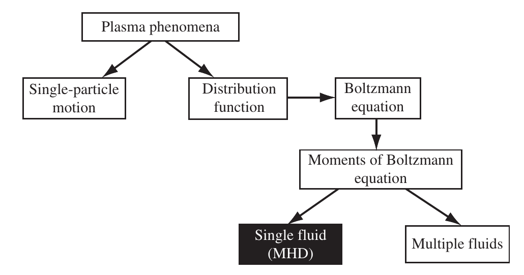
2.2 MHD plasma model

• Fluid description: it uses a few macroscopic quantities, averages of the distribution function (mean velocity, pressure/temperature). Valid for or near thermodynamic equilibrium.

2.3 Validity of the MHD model

Range of validity of different plasma codes based on typical magnetospheric parameters: \(n=50cm^{-3}\), \(B=50 nT\), \(T_e=T_i=100 eV\) (Winske and Omidi (1996)).

3 MHD equations

3.1 Approximation and definitions in single-fluid MHD

• Plasma is charge-neutral because \(L \gg \lambda_{de}\) (Poisson eq. is superfluous)
• \(V\ll c\) (no displacement current in Ampere’s)
• \(T\gg\Omega_{ce},\Omega_{ci}\) (electron/ion cyclotron frequencies)
• \(L\gg d_e, d_i\) (electron/ion skin depths) and \(L\gg \rho_e, \rho_i\) (electron/ion gyroradius) \[ \vec{J} = \sum_{\alpha}q_{\alpha}n_{\alpha}\vec{V}_{\alpha}\\ \vec{V}=\frac{1}{\rho}\sum_{\alpha}m_{\alpha}n_{\alpha}\vec{V}_{\alpha} \\ \rho = \sum_{\alpha} m_{\alpha}n_{\alpha} \]

3.2 Fluid equations

\[ \frac{\partial \rho}{\partial t} + \nabla\cdot(\rho \vec{V})=0 \] \[ \frac{\partial \rho \vec{V}}{\partial t} +\nabla\cdot(\rho \vec{V} \vec{V})= - \nabla\cdot\bar{P} + qn(\vec{E}+\vec{V}\times\vec{B}) \] \[ \frac{1}{\gamma - 1}\left( \frac{\partial \bar{P}}{\partial t} + \nabla\cdot(\bar{P}\vec{V}) \right) = -(\bar{P}\cdot\nabla)\cdot\vec{V} - \nabla\cdot\vec{L} \]

3.3 General algorithms

3.4 Fluid equations

• In fluid dynamics, we can write the equations for conservation of mass, momentum and energy as: \[ \frac{\partial\vec{q}}{\partial t} + \frac{\partial \bar{F}}{\partial x}= 0 \qquad(1)\] with \(\vec{q}\) and \(\bar{F}\) in 1D defined as \[ \vec{q}= \begin{pmatrix} \rho, & \rho V, & P/(\gamma -1) + (1/2)\rho V^2\end{pmatrix}^T\\ \vec{F}= \begin{pmatrix} \rho V, & \rho V^2 + P, & (\gamma P/(\gamma -1) + (1/2)\rho V^2)V \end{pmatrix}^T \] in 3D, \(\bar{F}\) is a 3x5 matrix (3 dimensions + 5 dependent variables, \(\rho\), \(P\), \(\vec{V}\))
• In many practical cases dissipative terms can be added to the terms in \(\bar{F}\), proportional to the derivatives \(\partial/\partial x\).
• MHD equations have the same structure with the additional equation and terms for the magnetic field.

3.5 MHD equations in conservative form

Conservative form of the MHD equations

\[ \frac{\partial \rho}{\partial t}= -\nabla \cdot\rho\vec{V} \\ \frac{\partial \rho \vec{V}}{\partial t}= -\nabla \cdot \left[\rho\vec{V}\vec{V} + \left(P + \frac{B^2}{2\mu_0}\right)\vec{1} - \frac{\vec{B}\vec{B}}{\mu_0}\right] \\ \frac{\partial \vec{B}}{\partial t} = \nabla\times\left[\vec{V}\times\vec{B}-\eta\vec{J}\right]\\ \frac{\partial w}{\partial t} = -\nabla \cdot \left[ \vec{V}\cdot\left(w + \left(P + \frac{B^2}{2\mu_0}\right) \right) -\frac{1}{\mu_0}(\vec{V}\cdot\vec{B})\vec{B} + \eta \vec{J}\times\vec{B} \right] \]

where the electric field, current density and total energy density are: \[ \vec{E} = - \vec{V}\times\vec{B} + \eta\vec{J} \\ \vec{J} = \nabla\times\vec{B}/\mu_0\\ w = \frac{1}{2}\rho V^2 + \frac{1}{2\mu_0} B^2 + \frac{P}{\gamma -1} \] \(\gamma=5/3\). Typical speeds: sound speed \(c_s=\sqrt{\gamma P/\rho}\), Alfv'en speed \(V_A=B/\sqrt{\mu_0 \rho}\).

3.6 Discretization for fluid equations

• Leapfrog: \[ \vec{q}_j^{n+1} = \vec{q}_j^{n-1} - \frac{\Delta t}{2\Delta x}(\vec{F}_{j+1}^n - \vec{F}_{j-1}^n) \]
• Lax-Wendroff: \[ \vec{q}_{j+1/2}^{*} = \frac{1}{2}\left(\vec{q}_j^{n} + \vec{q}_{j+1}^{n}\right) - \frac{\Delta t}{2\Delta x}(\vec{F}_{j+1}^n - \vec{F}_{j}^n)\\ \vec{q}_{j}^{n+1} = \vec{q}_j^{n-1} - \frac{\Delta t}{\Delta x}( \vec{F}_{j+1/2}^*-\vec{F}_{j-1/2}^*) \]
• Implicit scheme: Crank-Nicholson \[ \vec{q}_j^{n+1} - \vec{q}_j^{n} = - \frac{\Delta t}{4\Delta x}\left[ (\vec{F}_{j+1}^n - \vec{F}_{j-1}^n) + (\vec{F}_{j+1}^{n+1} - \vec{F}_{j-1}^{n+1}) \right] \]
• Note that all those schemes are 2nd order. Since dissipative terms involve second order derivatives, they should be treated via non-linear transport method or other discretizations for parabolic equations (e.g. DuFort-Frankel).

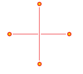
3.7 Methods for diffusion equations: Dufort-Frankel

• The Dufort-Frankel scheme is based on a modification of the FTCS scheme for the diffusion (parabolic) equation by using centered difference in time and the middle term in the Laplacian (\(2f_{j}^n\)) split into two time levels: \[ \frac{f_j^{n+1} - f_j^{n-1}}{2\Delta t} = \frac{\alpha}{\Delta x^2} L_{xx} f_j^n=\frac{\alpha}{\Delta x^2}(f_{j-1}^n - (f_{j}^{n-1} + f_{j}^{n+1}) + f_{j+1}^n ) \] and rearranging: \[ f_j^{n+1} = \frac{2s}{1+2s}(f_{j-1}^n + f_{j+1}^n ) + \frac{1-2s}{1+2s}f_{j}^{n-1} \]
• This scheme is unconditionally stable.

3.8 Flux conserving algorithms

• Grid points are considered cell centers at \(x_i\) (\(i=1,..N\)), while cell interfaces located at \(x_{i+1/2}=(x_i+x_{i+1})/2\) (\(N\) cell centers and \(N-1\) cell interfaces)
• We could consider the boundaries at \(x_{1/2}\) and \(x_{N+1/2}\), making a total of \(N+1\) cell interfaces.
• Let consider a 3D situation with the volume of each cell \(V=\Delta x S\) and \(S=\Delta y \Delta z\).
• the conserved quantity is \(q_i^N\), the total content in each cell is \(Q_i^n=q_i^n V\)
• Any change in the conserved \(Q_i^n\) must come from inflows and outflows through the cell interfaces via a flux \(f\): \[ \frac{dQ_i}{dt}\approx \frac{Q_i^{n+1} - Q_i^{n}}{\Delta t} =(f_{i-1/2}^{n+1/2} - f_{i+1/2}^{n+1/2})S \]
• Using the definitions of \(S\) and \(Q_i\), we get: \[ \frac{q_i^{n+1} - q_i^{n}}{\Delta t} =\frac{f_{i-1/2}^{n+1/2} - f_{i+1/2}^{n+1/2}}{\Delta x} \]
• The different flux conserving algorithms differ only in the calculation of \(f_{i\pm1/2}^{n+1/2}\) in terms of \(q_{i\pm}^{n}\) (e.g., Donor-cell advection, piecewise linear schemes, flux-limiter methods), and the methods are usually called Finite Volume Methods.

3.9 Finite Volume Methods

• Those methods are not applied to the equations in conservation form, but rather on their integral form.
• The computational domain is subdivided into a finite number of contiguous volumes (e.g.: cuboids) and the quantities are calculated at the centroid.
• The surfaces of those volume are used for the integral conservation relations, while derivatives are transformed via Gauss divergence theorem.
• Example: \[ \left( \frac{\partial \phi}{\partial x}\right)= \frac{1}{\Delta V}\int_{\Delta V} \frac{\partial \phi}{\partial x}d^3x=\frac{1}{\Delta V}\int_{\partial V}\phi dS^x\approx \frac{1}{\Delta V}\sum_{j=1}^N \phi_j S_j^x \] where \(\phi_j\) are the values of the function at the surfaces and \(N\) is the number of bounding surfaces of the volume.

4 MHD applications

4.1 MHD applications

4.2 Typical MHD code

• The numerical simulation results to be shown were generated with a MHD code developed mainly for magnetospheric applications (credits: A. Otto). The latest 3D parallel version is described by Skála et al. (2015), and it is mainly used for solar coronal simulations.
• Accuracy: second order, discretization using the Leapfrog (for the conservative part) - Dufort-Frankel method (for the dissipative terms). Option to also use Lax-Wendroff.
• In order to avoid grid-oscillations due to the Leapfrog method, numerical diffusion \(\propto \nabla^2\) is added to the right hand side of the MHD equations.

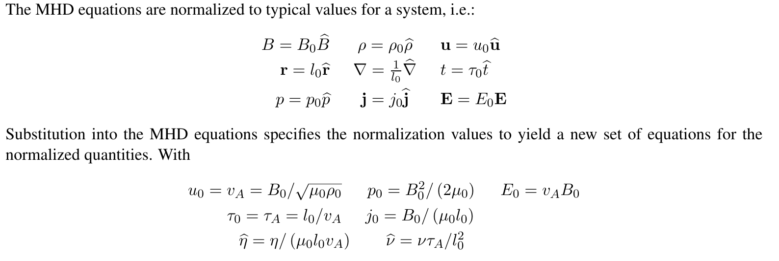
4.3 Normalizations

• Typical input normalization values: \(L_0=400 km\), \(B_0=50 nT\), \(n_0=7.5 cm^{-3}\) computed in the code: \(V_0\), \(P_0\), \(T_0\).
• The velocity normalization is the Alfvén speed: \(V_0=B_0/\sqrt{\mu m_pn_0}\)
• The time normalization is the Alfvén transit time \(T_0=L_0/V_0\)
• The pressure is normalized to the magnetic pressure \(P_0=B_0^2/2\mu_0\)

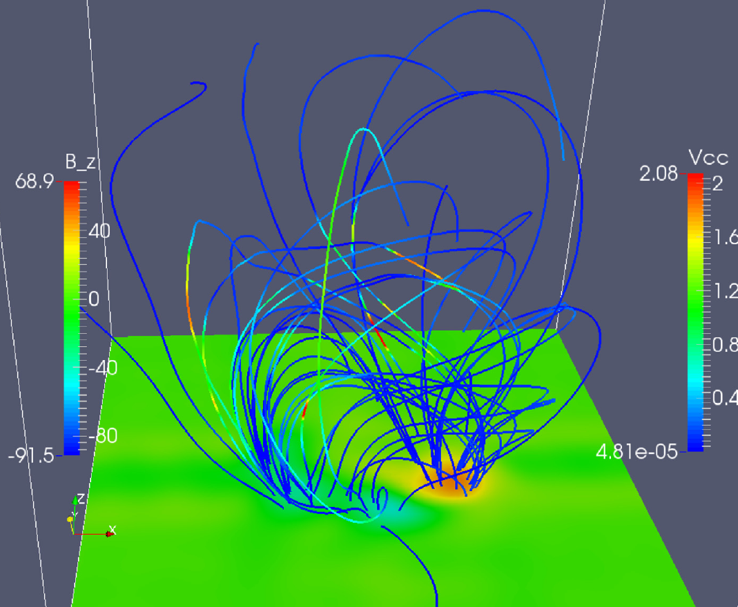
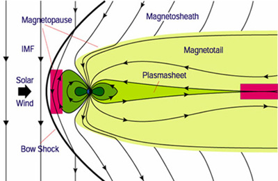
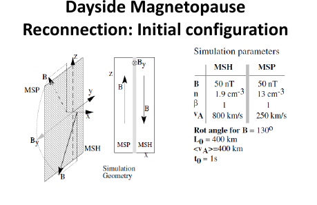
4.4 Example 1: Magnetotail reconnection

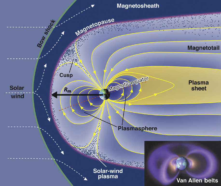
4.5 Example 1: Magnetotail reconnection

4.6 Example 1: Magnetotail reconnection

https://www.youtube.com/watch?v=mgUZwoR0gcE

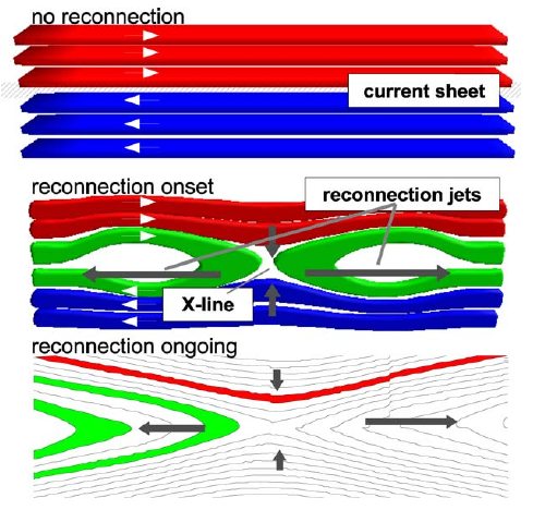
4.7 Magnetic reconnection

4.8 Example 1.5: Tearing instability

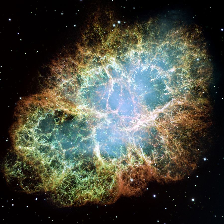
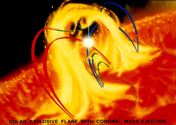
4.9 Magnetic reconnection in the Sun

4.10 Example 2: Magnetopause Kelvin-Helmholtz instability

4.11 Example 2: Magnetopause Kelvin-Helmholtz instability

• Growth rate: \[ q=\sqrt{\alpha_1 \alpha_2[(\vec{V}_1 - \vec{V}_2)\cdot\vec{k}] - \alpha_1(\vec{V}_{A1}\cdot\vec{k})^2 - \alpha_1(\vec{V}_{A2}\cdot\vec{k})^2 } \] where \(\alpha_i=\rho_i/(\rho_1 + \rho_2)\) and \(\vec{V}_{Ai}=\vec{B}/\sqrt{\rho_i}\) is the Alfv'en speed
• For \(B=0\), KH is always operative as long as there is a shear \((\vec{V}_1 - \vec{V}_2)\neq 0\)
• Strong enough \(B\) along \(k\) can stabilize KH.

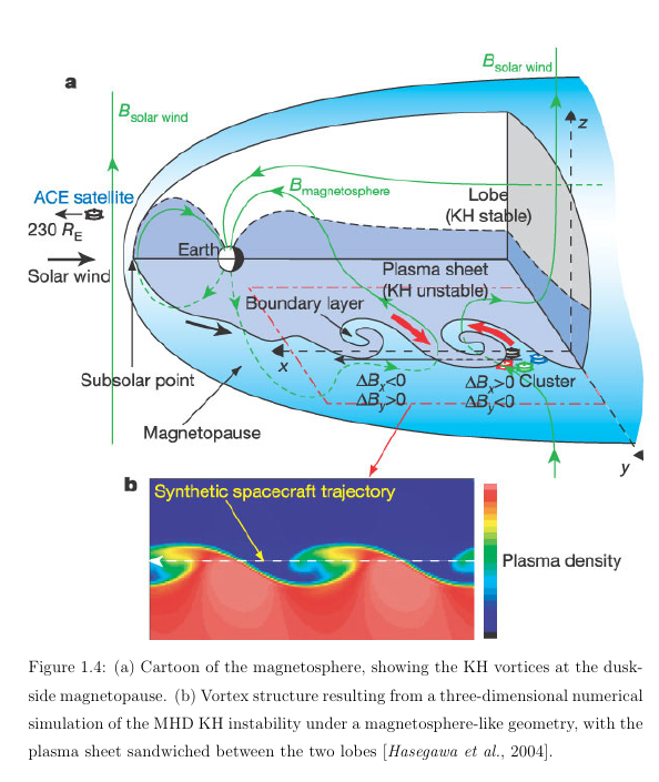
4.12 Example 2: Magnetopause Kelvin-Helmholtz instability

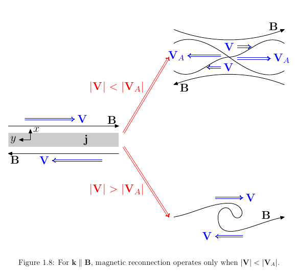
• Magnetic reconnection and KH can interact in realistic scenarios: e.g.: shear flows in magnetopause reconnection
• For shears flows \(V>V_A\), magnetic reconnection is switched off by KH modes.

4.13 Example 2: Magnetopause Kelvin-Helmholtz instability

4.14 Example 2: Kelvin-Helmholtz instability

5 Example 3: Rayleigh-Taylor instability

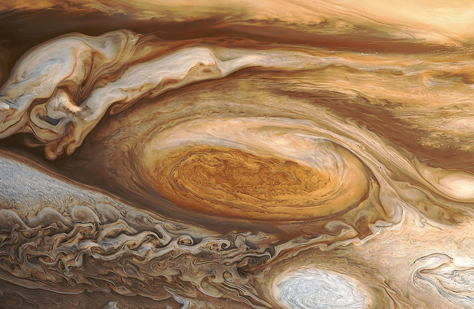
5.1 Rayleigh-Taylor instability

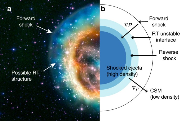
5.2 Rayleigh-Taylor instability

5.3 Popular astrophysical MHD codes

• Pencil: https://github.com/pencil-code/pencil-code
• ENZO: https://github.com/enzo-project/enzo-dev, Bryan et al. (2014)
• ATHENA++: https://github.com/PrincetonUniversity/athena, James M. Stone et al. (2008),James M. Stone et al. (2020)
• RAMSES: https://bitbucket.org/rteyssie/ramses/wiki/Home, Masson et al. (2012)
• NIRVANA: https://gitlab.aip.de/ziegler/NIRVANA Ziegler (2008)
• PLUTO: http://plutocode.ph.unito.it, Mignone et al. (2012)
• MPI-AMRVAC 2.0: https://github.com/amrvac/amrvac, Xia et al. (2018)
• CRONOS: https://www.uibk.ac.at/astro/research_groups/ralf-kissmann/home/cronos-code.html, Kissmann et al. (2018)

5.4 References

Bryan, Greg L, Michael L Norman, Brian W. O’Shea, Tom Abel, John H Wise, Matthew J Turk, Daniel R Reynolds, et al. 2014. “ENZO: AN ADAPTIVE MESH REFINEMENT CODE FOR ASTROPHYSICS.” Astrophys. J. Suppl. Ser. 211 (2): 19. https://doi.org/10.1088/0067-0049/211/2/19.

Kissmann, R., J. Kleimann, B. Krebl, and T. Wiengarten. 2018. “The CRONOS Code for Astrophysical Magnetohydrodynamics.” Astrophys. J. Suppl. Ser. 236 (2): 53. https://doi.org/10.3847/1538-4365/aabe75.

Masson, J, R Teyssier, C. Mulet-Marquis, P Hennebelle, and G Chabrier. 2012. “INCORPORATING AMBIPOLAR AND OHMIC DIFFUSION IN THE AMR MHD CODE RAMSES.” Astrophys. J. Suppl. Ser. 201 (2): 24. https://doi.org/10.1088/0067-0049/201/2/24.

Mignone, A, C Zanni, P Tzeferacos, B. van Straalen, P Colella, and G Bodo. 2012. “THE PLUTO CODE FOR ADAPTIVE MESH COMPUTATIONS IN ASTROPHYSICAL FLUID DYNAMICS.” Astrophys. J. Suppl. Ser. 198 (1): 7. https://doi.org/10.1088/0067-0049/198/1/7.

Skála, J., F. Baruffa, Jörg Büchner, and M Rampp. 2015. “The 3D MHD code GOEMHD3 for astrophysical plasmas with large Reynolds numbers.” Astron. Astrophys. 580 (25274): A48. https://doi.org/10.1051/0004-6361/201425274.

Stone, James M, Thomas A Gardiner, Peter Teuben, John F Hawley, and Jacob B Simon. 2008. “Athena: A New Code for Astrophysical MHD.” Astrophys. J. Suppl. Ser. 178 (1): 137–77. https://doi.org/10.1086/588755.

Stone, James M., Kengo Tomida, Christopher J. White, and Kyle G. Felker. 2020. “The Athena++ Adaptive Mesh Refinement Framework: Design and Magnetohydrodynamic Solvers.” The Astrophysical Journal Supplement Series 249 (1): 4. https://doi.org/10.3847/1538-4365/ab929b.

Winske, D., and N. Omidi. 1996. “A nonspecialist’s guide to kinetic simulations of space plasmas.” J. Geophys. Res. 101 (A8): 17287. https://doi.org/10.1029/96JA00982.

Xia, C., J. Teunissen, I. El Mellah, E. Chané, and R. Keppens. 2018. “MPI-AMRVAC 2.0 for Solar and Astrophysical Applications.” Astrophys. J. Suppl. Ser. 234 (2): 30. https://doi.org/10.3847/1538-4365/aaa6c8.

Ziegler, U. 2008. “The NIRVANA code: Parallel computational MHD with adaptive mesh refinement.” Comput. Phys. Commun. 179 (4): 227–44. https://doi.org/10.1016/j.cpc.2008.02.017.