Lecture 10: High performance computing – Lecture

Jan Benáček

Institute for Physics and Astronomy, University of Potsdam

January 16, 2025

1 Lecture overview

Table of Contents 1/2

17.10. Introduction + numerical methods summary
24.10. Numerical methods of differential equations — lecture + hands-on
31.10. State holiday
07.11. Test particle approach — lecture
14.11. Test particle approach — lecture + hands-on
21.11. PIC method — lecture
28.11. PIC method — hands-on

Table of Contents 2/2

05.12. Fluid and MHD — lecture (online)
12.12. Fluid and MHD — hands-on given Xin-Yue Shi
19.12. Canceled
09.01. Radiative transfer — lecture + hands-on
16.01. HPC computing — lecture + hands-on
23.01. Advanced — Smooth particle hydrodynamics method — lecture
30.01. Advanced — Hybrid, Gyrokinetics — lecture
06.02. Advanced — Vlasov and Linear Vlasov dispersion solvers — lecture

2 High performance computing (HPC) introduction

2.1 Introduction

Definition of High performance computing (HPC)

Usage of supercomputers and computer clusters to solve advanced computation problems.

Simple performance estimation

Let us assume, we have numerically implemented one of the space plasma simulation algorithms.
What is the simulation performance at a typical computer?

4 cores at 5 GHz, calculating 4 floating point operations (Flops) at CPU tick \(\Rightarrow\) 80 GFlops.

What can we achieve?
Pushing one particle per one time step can take 100 Flops \(\Rightarrow\) pushing 800 M particles per second (in ideal case).

2.2 Your turn

Do we need higher performance? Why?
How can we speed up?
What can go wrong in my calculation?
Have you used any computer cluster?
If yes, which one and to calculate what?
Did you hear about supercomputer “fights” between countries?
Do you plan to follow the academic path after finishing your degree?
Do you consider to start working in industry after finishing your degree?

3 Examples of supercomputers

3.1 Top500

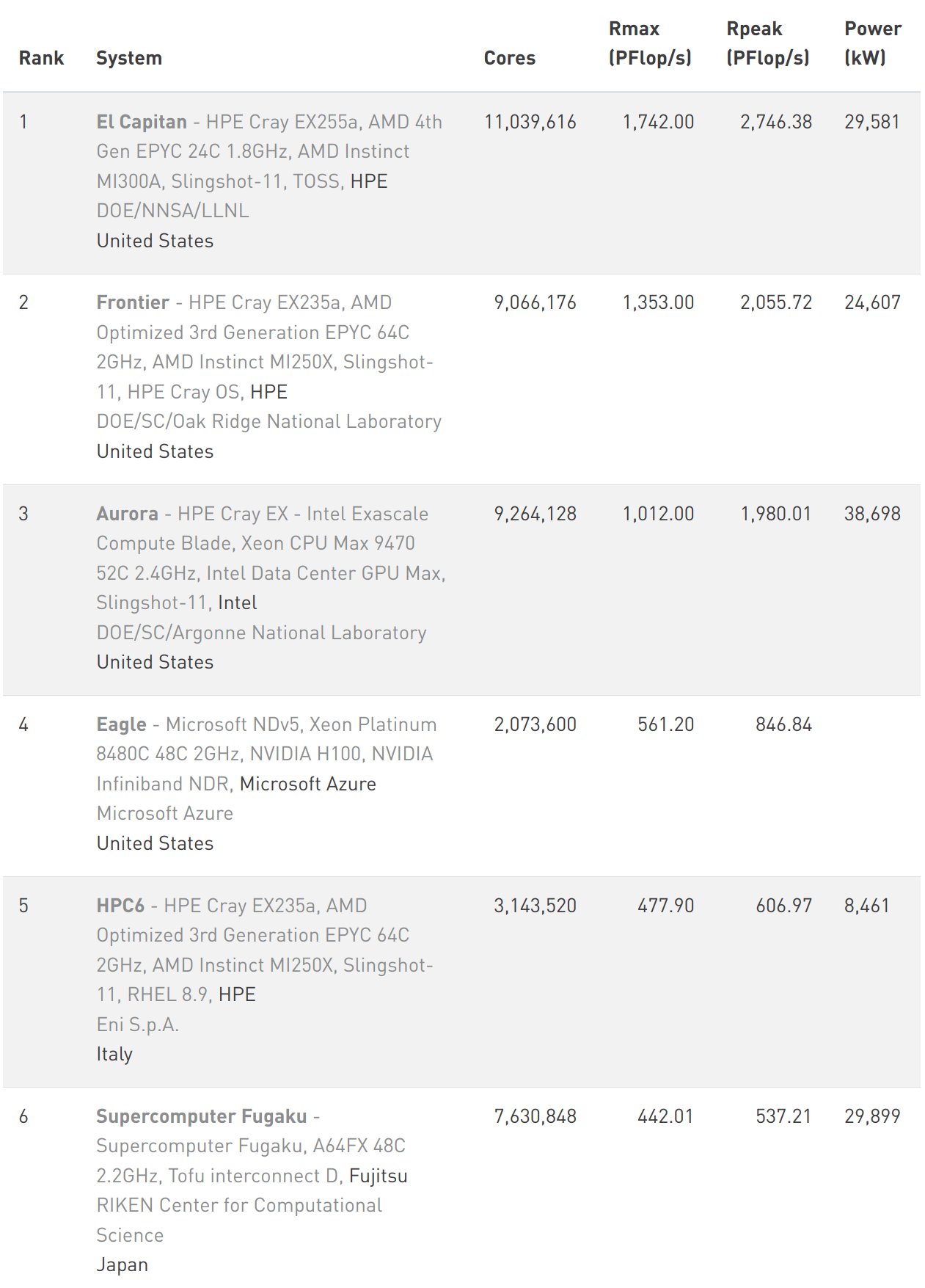
List of the most powerfull supercomputers in the world: Top 500
Released every half-year, now November 2024 release
Not all computers are listed

3.2 Examples

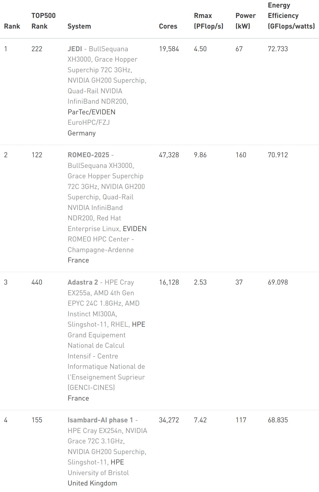
3.3 Green500

List of the most energy efficient supercomputers in the world:
Green500

3.4 Quantum computing

IQM quantum computers

3.5 Distributed vs cloud computing

Figure

3.6 Access to a (super)computer

Postdam Uni offers: HPC cluster for all members: Getting access
Gauss center for supercomputing — Hawk, JUWELS, and SuperMUC-NG
IT4I in Ostrava, CZ - Karolina, Barbora
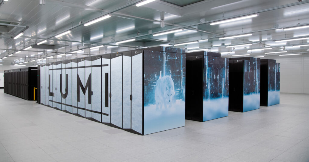
EuroHPC - LUMI, Leonardo, many others
Many cluster offer free! training activities: EuroHPC, Gauss center — typicaly from very basic up to very advanced

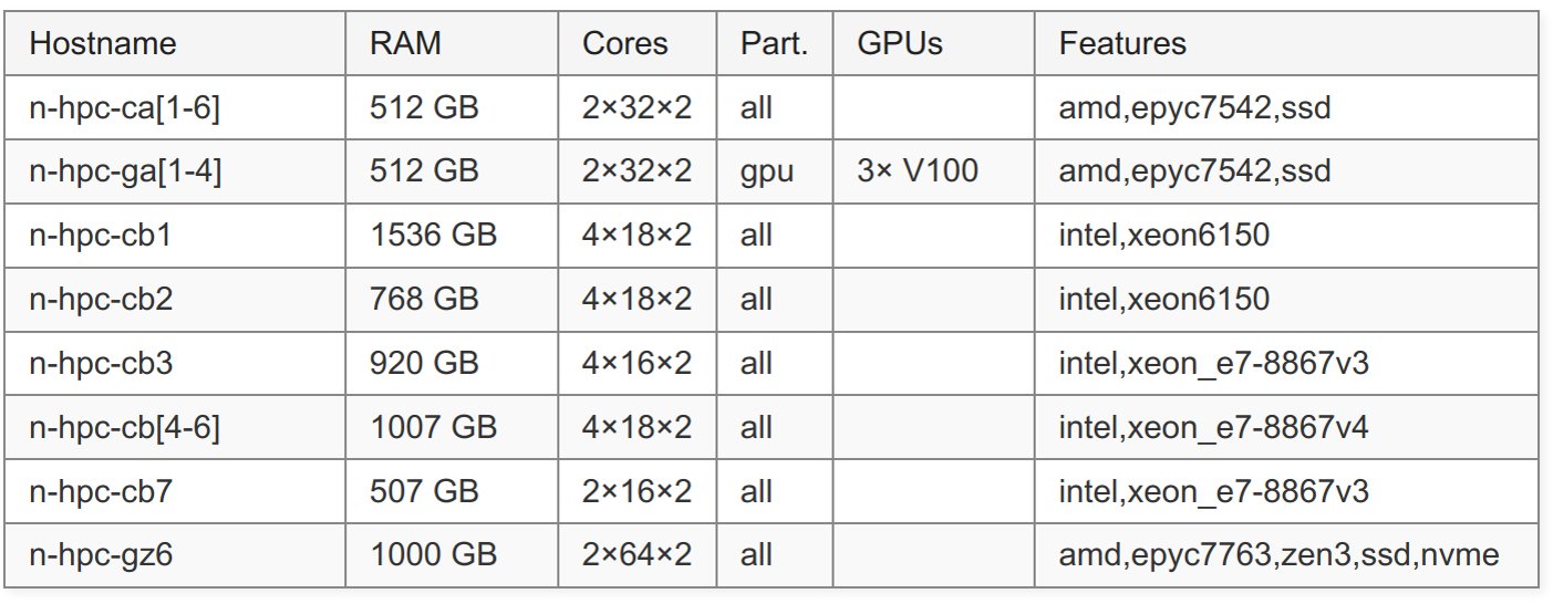
Node List of Uni Potsdam cluster

3.7 Application procedure to cluster

Profile you simulation that it really well scales with number of CPUs or GPUs
Find an interesting large-scale simulation research
Write an application and apply at the center
Do (not) obtain computing time
Access the cluster, compile your simulation, upload your data
Submit jobs to queue
Wait! for running
Process, analyze, and download your data

4 Inside the supercomputer

4.1 Supercomputer scheme

Scheme of a MeluXina supercomputer (Luxembourg)

4.2 Front-nodes / Access nodes

Access to the cluster
Typically connected through SSH (Secure SHell)
Not for computing porposes
Usefull for data upload/download, easy analysis, visualization,…
Code compilaton, Running Jupyter Lab, Paraview, Job submission

4.3 Compute nodes

Unit determined for the calculations
Typically not accessible for a user directly, automatic processing using job queue
Large computing power
Various types of nodes can be present at the supercomputer
- Compute nodes (typically 2 CPUs with 96 cores and 128 GB RAM)
- Fat nodes (typically 8 CPUs with 256 cores and 1 TB RAM)
- Testing nodes
- GPU/Accelerated/CPU nodes (typically 2 CPUs and 128 GB RAM, 6 GPUs and 384 HBM memory )

4.4 Storage

Large scale storage for simulation outputs
Always good to know the properties
Local storage at nodes / Commong storage for whole cluster
To upload/download large data (>TBs), specific transport protocols available, like GLOBUS)
Usual topology:
- Scratch - direct output from simulations, fast
- Work - data processing, fast
- Archive - long-term data backup, tapes, slow
Each typically tens of PBs of data

4.5 Infiniband

To get more nodes cooperating at calculation of the same simulation
It provides connection and communication between nodes and between nodes and storages
Extremely fast (~400 Gbps between each two nodes) + huge aggregated bandwidth
Extremely low latency (~1\(\mu\)s)
For comparison, fast ethernet can reach ~100 Gbps and 1 ms latency
Simulations must be prepared to used this communication - Message Passing Interface (MPI)

4.6 Software

Operating system
Modules
Licenses
Containers
Compilation
Analysis

4.7 SuperMUC-NG Queues

4.8 Example of SuperMUC-NG - My Hands-on session

5 Simulation on a PC/node

5.1 How our computers compute our simulations?

In the following slides, various ways how the computer are optimized to run as fast as possible
This understanding can help to speed-up our codes
Several hardware + software levels
Hardware for calculations: CPUs + GPUs + Other accelerators
Software speed-up techniques: OpenMP, MPI, CUDA, HIP, …

5.2 CPUs

5.3 CPU - Central Processing Unit

Basic and general-purpose processing unit of a computer
Reads the instructions of binary programs and executes them
Advantage: can run various programs and types of loads, prepared be the control unit of a computer
Disadvantage: Not many calculations can be done in parallel
Execution speed approx. the clock speed (typically a few GHz)
Two main techniques how to speed-up:
1. Instruction level parallelism
2. Task level parallelism

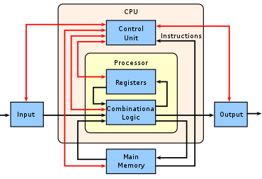
Scheme of a CPU Wiki.

5.4 Pipelines

Every instruction of a program has several phases
Pipeline: Load/Fetch instruction -> Decode -> (Load data) -> Execute -> Memory Access -> Write Back -> …
This loop can be parallelized
Different unit for each step
E.g., when one instruction get decoded, next one can be already loaded.

Pipeline

5.5 Superscalarity

Each step in the pipeline can be also done in parallel
Specific ones for floating point, integer, load, store operations
Some pipeline items present more times
Different execution times for integer: add (1 cycle); double: add (4 cycles), multiply (7), divide (23), sqrt(>23).
Not every instruction takes the same place (a few to thousands of clock ticks)

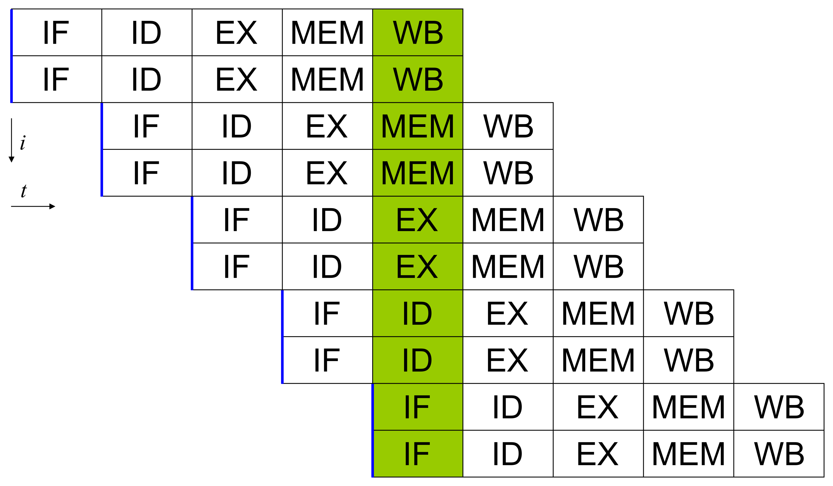
Superscalar pipeline

5.6 Vector Instructions

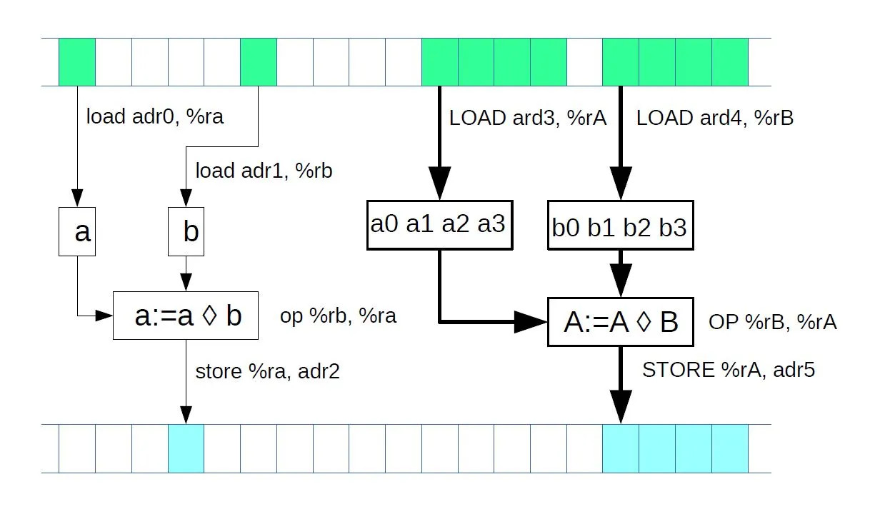
To process even more data a time, each instruction can take more scalar values
E.g., AVX512 instructions can take 8 Double scalars. The mathematical operation is simultaneous at all 8 numbers
Advantage: increased performance up to 8 times
Disadvantages:
- Large memory transports - large bandwidth required
- Not all processors support all types of vector operations
- The code (e.g., a loop) must be able to process data independently

Vector instructions

5.7 Threads — Hyperthreading

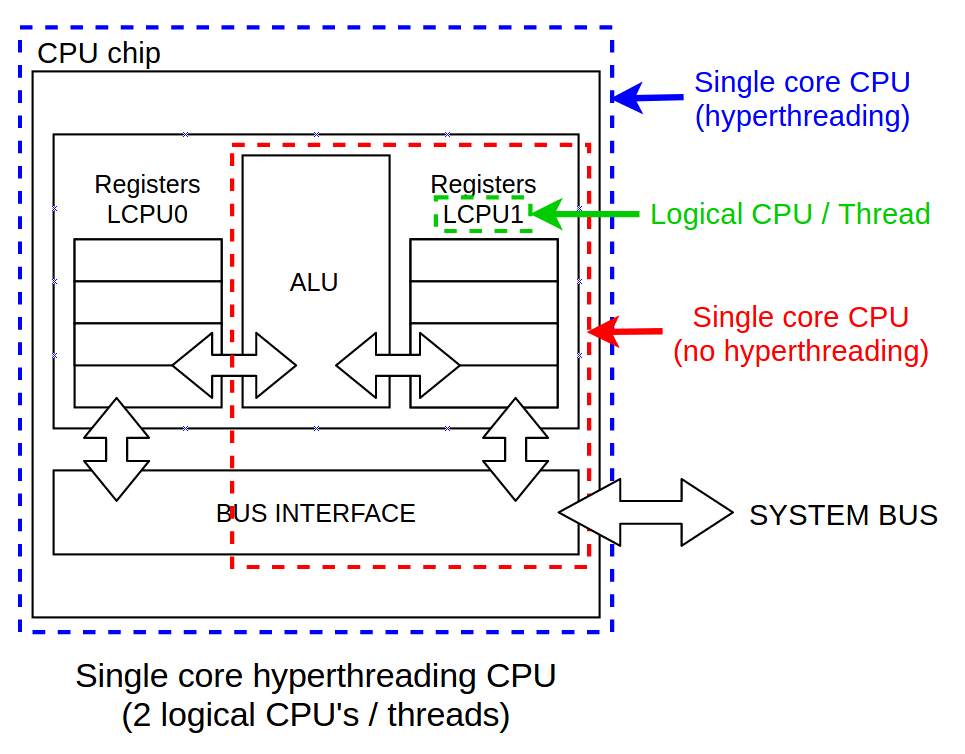
To efficiently utilize all execution units, each core can run two or more independent threads
The threads are indipendent programs, but they utilize the same execution units
If the execution units not utilized, they would only wait and consume energy

Hyperthreading

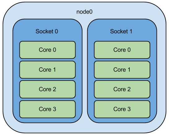
5.8 Cores

Implementing more independent cores mean more programs can run in parallel
However, if more programs solve the same issue, they have to communicate
Communication between cores is relatively slow (~100 clock ticks)
Also, the programs must be prepared (by programmer) to run more time and communicate to each other
If not prepared, the parallel run at more cores is basically not possible

Node Topology

5.9 GPUs

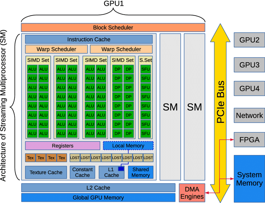
5.10 GPU - Graphical Processing Unit

Originally developed for computer games
Advantage: Relatively narrow-purpose unit to run as many simultaneous calculations as possible.
Disadvantage: The programs must be prepared to take into account many execution units; if not, the program is running very inefficient way (and lots of power and money burned)
Typical tick speed of 2 GHz
Each multiprocessors many parallel execution units called stream processors
Typical power: 16000 stream processors x 2 GHz = 32 TFlops (4 core CPU has 200-1000 GFlops)

Scheme of a GPU

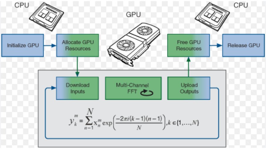
5.11 GPU acceleration — offloading

Start our program on CPU
Send the calculation to GPU
Obtain the results from GPU
Store/finish the simulation on CPU

GPU offloading

5.12 Memory management

5.13 Memory management

Differences between CPU and GPU
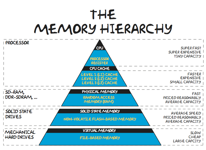
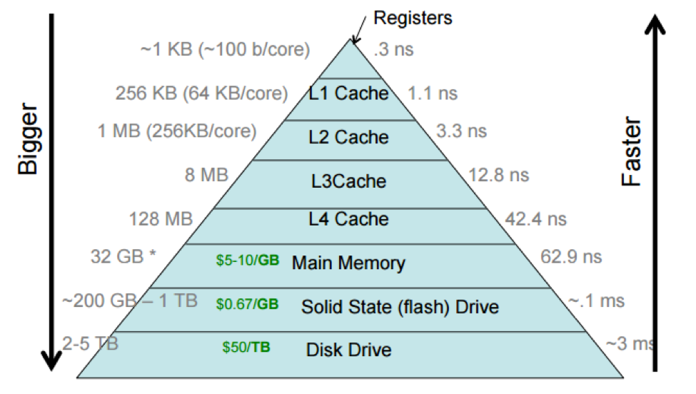
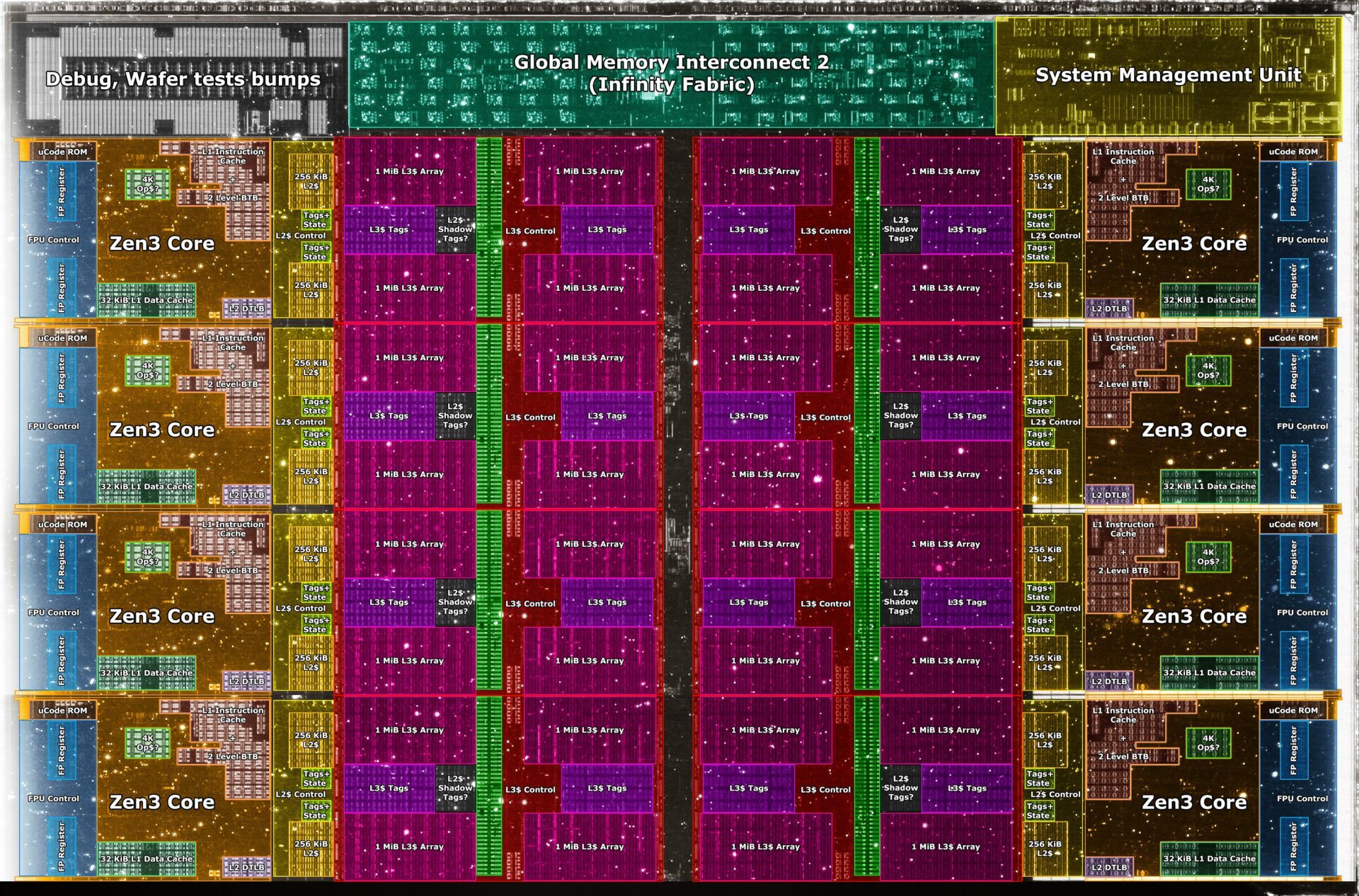
Scheme how data flow from RAM to L3, L2, L1 to L0 and execution unit
Various times to transport the data \(\Rightarrow\) the best approach is to keep the programm to close to the core as possible
Do not make dependent loops, if the program has to wait to something previous, it cannot proceed.
Memory vs. Computing bound tasks

5.14 AMD Ryzen Die Scheme

Die scheme

5.15 Test the performance

We want to utilize the CPU as much as possible during our calculations
Compare the following cases in Jupyter notebook

N = 1_000_000
a = np.random.random(N)
b = np.random.random(N)
c = np.zeros_like(a)

%%timeit
for i in range(N):
    c[i] = a[i] + b[i]

231 ms ± 17.2 ms per loop (mean ± std. dev. of 7 runs, 1 loop each)

%%timeit
c = a + b

1.1 ms ± 83.9 µs per loop (mean ± std. dev. of 7 runs, 1,000 loops each)

6 Parallelization techniques

6.1 OpenMP — Open Multi-Processing

Easiest way to run your program parallel
Work only in some compiled languages — C/C++ and Fortran
Maximal parallelization limited to one CPU

Example:

int a[100000];

for (int i = 0; i < 100000; i++) {
    a[i] = 2 * i;
}

Is transformed to

int a[100000];

#pragma omp parallel for
for (int i = 0; i < 100000; i++) {
    a[i] = 2 * i;
}

6.2 MPI — Message Passing Interface

Communication protocol between processes
A standard for supercomputer processing
Utilization of all nodes at the cluster
The communication must be implemented into the current simulation code
Example

Initialization and finishing

    // Initialize the MPI environment
    MPI_Init(NULL, NULL);

    // Get the number of processes
    int world_size;
    MPI_Comm_size(MPI_COMM_WORLD, &world_size);

    // Get the rank of the process
    int world_rank;
    MPI_Comm_rank(MPI_COMM_WORLD, &world_rank);

    // Print off a hello world message
    printf("Hello world from processor rank %d out of %d processors\n",
           world_rank, world_size);

    // Finalize the MPI environment.
    MPI_Finalize();

Communication

int number;
if (world_rank == 0) {
    number = -1;
    MPI_Send(&number, 1, MPI_INT, 1, 0, MPI_COMM_WORLD);
} else if (world_rank == 1) {
    MPI_Recv(&number, 1, MPI_INT, 0, 0, MPI_COMM_WORLD,
             MPI_STATUS_IGNORE);
    printf("Process 1 received number %d from process 0\n",
           number);
}

Compilation and run

mpicc -o hello_world hello_world.c
mpirun -n 4 hellow_world

6.3 CUDA/HIP

Used for offloading to the GPUs
More ways how to do it
OpenACC or OpenMP offloading
- similar to OpenMP but more directives
- Not so good performance
- Not broadly supported
CUDA/HIP
- Your code must be rewritten to a different programming language
- Excellent performance can be reached
- Running on NVIDIA or AMD GPUs
- Using so called kernels - peaces of code that can run in parallel

6.4 CUDA Example

void c_hello(){
    printf("Hello World!\n");
}

int main() {
    c_hello();
    return 0;
}

CUDA

__global__ void cuda_hello(){
    printf("Hello World from GPU!\n");
}

int main() {
    cuda_hello<<<1,1>>>(); 
    return 0;
}

6.5 Others

Other accelerator types exist
The mostly used are FPGAs — Field-programmable gate array
A microprocessor/array that can be setup at the beginning and than run only that calculation
Extremely fast calculations
Difficult to program