Lecture 11: Smooth Particle Hydrodynamics – Lecture + Hands-on

Jan Benáček

Institute for Physics and Astronomy, University of Potsdam

January 23, 2024

1 Lecture overview

Table of Contents 1/2

17.10. Introduction + numerical methods summary
24.10. Numerical methods of differential equations — lecture + hands-on
31.10. State holiday
07.11. Test particle approach — lecture
14.11. Test particle approach — lecture + hands-on
21.11. PIC method — lecture
28.11. PIC method — hands-on

Table of Contents 2/2

05.12. Fluid and MHD — lecture (online)
12.12. Fluid and MHD — hands-on given Xin-Yue Shi
19.12. Canceled
09.01. Radiative transfer — lecture + hands-on
16.01. HPC computing — lecture + hands-on**
23.01. Advanced — Smooth particle hydrodynamics method — lecture
30.01. Advanced — Hybrid, Gyrokinetics — lecture
06.02. Advanced — Vlasov and Linear Vlasov dispersion solvers — lecture

2 Introduction

2.1 Properties of SPH

Lagrange methods
Particles representing a part of plasma/fluid
Mesh-less

2.2 Kernel function

Kernel function describes a smooth quantity by weighting macro-particles
Similar to PIC weighting/smooth function of macro-particles \[ f(\vec{x}) = \int_{\Omega} f(\vec{y}) W(\vec{x} - \vec{y}, h) d\vec{y} \]
$h$ is the smoothing length
for $h \rightarrow$ 0, $W$ approach delta function
for $|\vec{r}| > K_{max} h$, we define $W(\vec{r}) = 0$

SPH kernel function (DOI).

2.3 Kernel function

The field $f$ is obtained by discretization into macro-particles
Macro-particles have mass $m_i$, density $\rho_i$, and volume $V_i = m_i / \rho_i$
In the most simple (fluid) case, each macro-particles has position $\vec{i}$, velocity $\vec{v}_i$
For a finite number of macro-particles, the kernel is expressed as \[ f(\vec{x}_i) = \sum_{j} V_j f(\vec{x}_j) W(\vec{x}_i - \vec{x}_j, h) \]
For example, fluid density is \[ \rho(\vec{x}_i) = \sum_{j} m_j W(\vec{x}_i - \vec{x}_j, h). \]

3 Equations of motion

3.1 Equations of motion

Using SPH approach to discretize fluid equations of motion
In Lagrangian form \[ \frac{d \rho}{dt} = - \rho \nabla \cdot \vec{u} \] \[ \frac{d\vec{u}}{dt} = - \frac{1}{\rho} \nabla p + \nu \nabla^2 \vec{u} + \vec{g} \]
$p$ is the pressure
$\rho$ is the density
$\nu$ is the kinematic viscosity
$\vec{g}$ is the acceleration due to the external force

3.2 Weakly compressible fluid

In weakly compressible fluid (not typical for astrophysics), equation of state is \[ p = \frac{c_0^2 \rho_0}{\gamma} \left[ \left( \frac{\rho}{\rho_0} \right)^\gamma - 1 \right] \]
$= 7 $ is the adiabatic index
$\rho_0$ - reference density (to which we assume the perturbation
$c_0$ is the sound speed (for the reference density)

3.3 Discrete form of equations of motion

Then, the equations of motion get form \[ \frac{d \rho_i}{dt} = \sum_j m_j (\vec{v}_i - \vec{v}_j) \cdot \nabla_i W_{i,j} \] \[ \frac{d\vec{u}_i}{dt} = \vec{a}_p + \vec{a}_{visc} + \vec{a}_{body} \] where \[ \vec{a}_p = - \sum_j m_j \left( \frac{p_i}{\rho_i^2} + \frac{p_j}{\rho_j^2} \right) \nabla_i W_{i,j} \] is the acceleration due to other particles.
$p_i$ is the pressure on $i$-th particle created by pressure $p_j$ of $j$-th particle
$\nabla_i W_{i,j} = \frac{\partial W (\vec{x}_i - \vec{x}_j, h)}{\partial \vec{x}_i}$ is the gradient of the kernel function.

3.4 Discrete form of equations of motion

\[ \vec{a}_{visc} = \sum_j m_j \frac{4\nu}{(\rho_i + \rho_j)} \frac{\vec{r}_{i,j} \cdot \nabla_i W_{i,j}}{(|\vec{r}_{i,j}|^2 + \eta h^2)} \vec{u}_{i,j} \] is the acceleration due to viscous forces
$\vec{r}_{i,j} = \vec{x}_i - \vec{x}_j$
and $\vec{a}_{body}$ is the acceleration due to external force.
Particle positions are obtained by \[ \frac{d\vec{x}_i}{dt} = \vec{u}_i \]
Some boundary conditions should be considered.

4 Numerical algorithms

4.1 Particle push — particle time integration

Typically, predictor-corrector scheme is used:
1. \[ \vec{u}_i^{n + \frac{1}{2}} = \vec{u}_i^n + \frac{\Delta t}{2} \left( \frac{d \vec{u}_i}{dt} \right)^n, \]
2. \[ \vec{x}_i^{n+1} = \vec{x}_i^n + \Delta t \vec{u}_i^{n + \frac{1}{2}}, \]
3. \[ \vec{u}_i^{n+1} = \vec{u}_i^{n+\frac{1}{2}} + \frac{\Delta t}{2} \left( \frac{d \vec{u}_i}{dt} \right)^{n+1}. \]
CFL condition must be fulfilled \[ \Delta t < \frac{\Delta x}{c}. \]
Implicit schemes are not usual.

4.2 Search of nearest neighbor particles

The methods would be extremely computational demanding if all particles interact with each other
For motion of each particle, we need to know the neighboring particles that influence its motion
These algorithms are known as ‘’nearest neighbor particles search’’ (NNPS)
Used also in many other computational disciplines like computational chemistry, engineering, …

4.3 How it works:

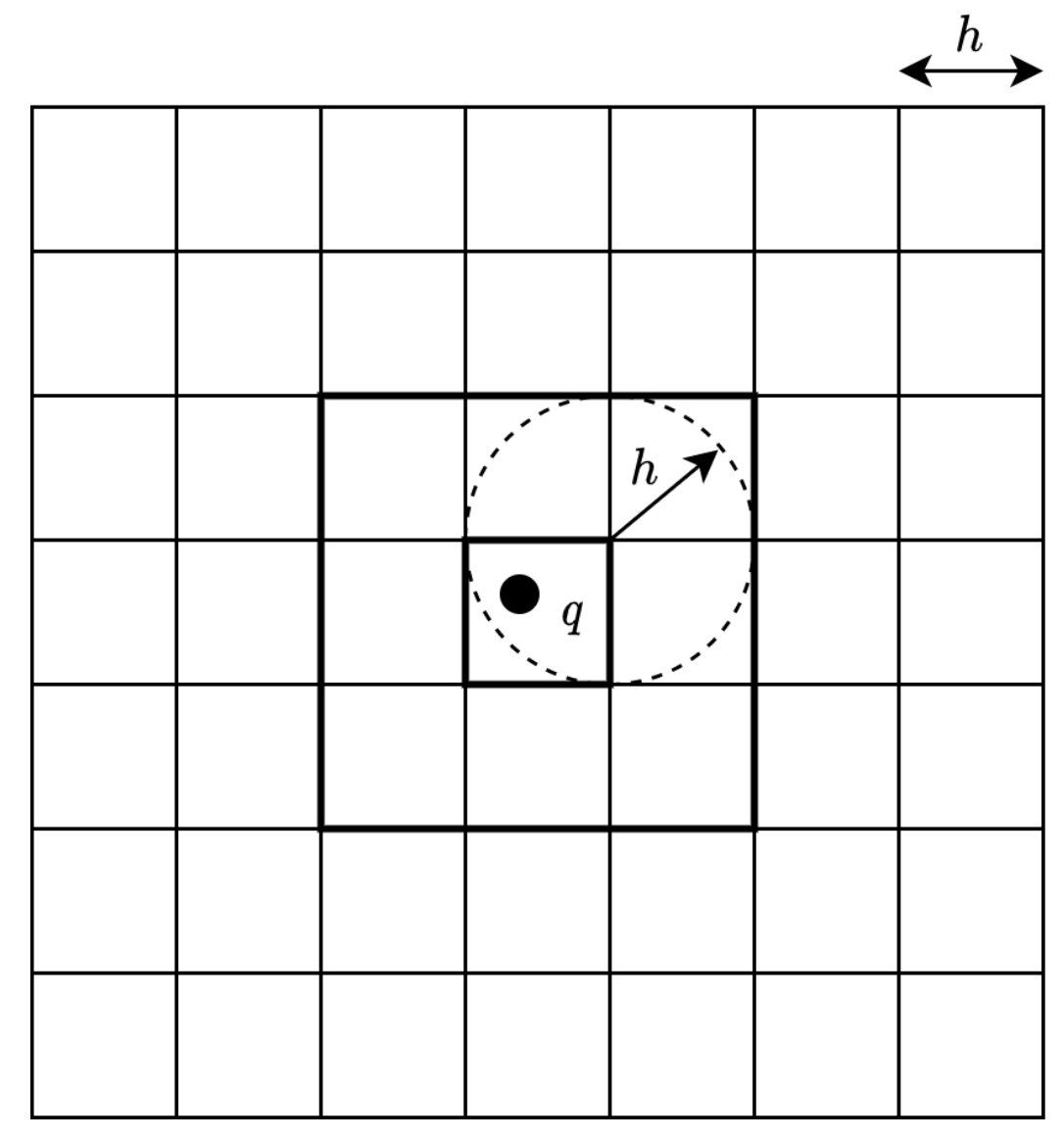
Particle are devided into cells of an uniform grid
The grid size is the particle radius (for various particles radii, the largest must be used)
Neighbors are always the particles in surrounding boxes
Works well for constant particle radii

NNPS

4.4 NNPS for variable radii

When particles can change their radii, some cells contain only a few particles while other really many
Various data structures were proposed to efficiently handle particle neighbors
Options:
- Octree - Widely used; divide the 3D grid cell into 8 octants into subgrids untill the subgrid has less than specified number of particles; well for parallelization; manipulation with subgrids not so easy.

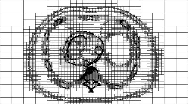
Octree algorithm DOI.

4.5 Linked list

Mapping each cell to an ID which is mapped into a head array of particles-
The head array stores the first particle of that cell
There is second array that maps the next particle;
Better cache performance, but needs to allocate large array.

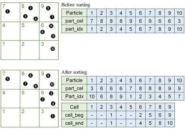
Linked list (DOI)

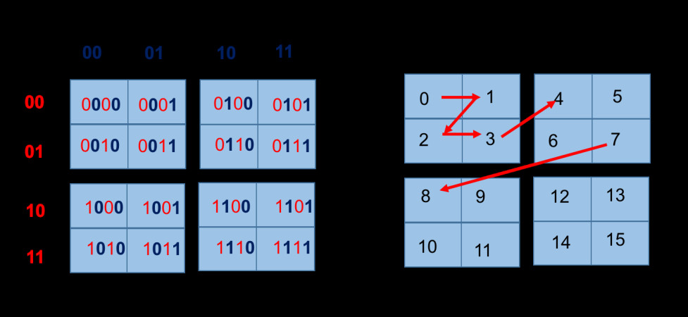
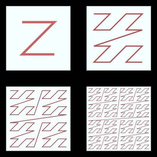
4.6 Z-Order Space Filling Curve

Create a spatial order of surrounding particles;
Sorting particles order based on their localization;
This way close particles in space are close in the list.

5 SPH examples

5.1 Non-astrophysical examles of fluids

Fluid examples
Comparison of water and SPH fluid evolution
Tutorial - Play close to time 43:50
Some fun

5.2 Astrophysical examples

5.3 Simulations of Galaxies

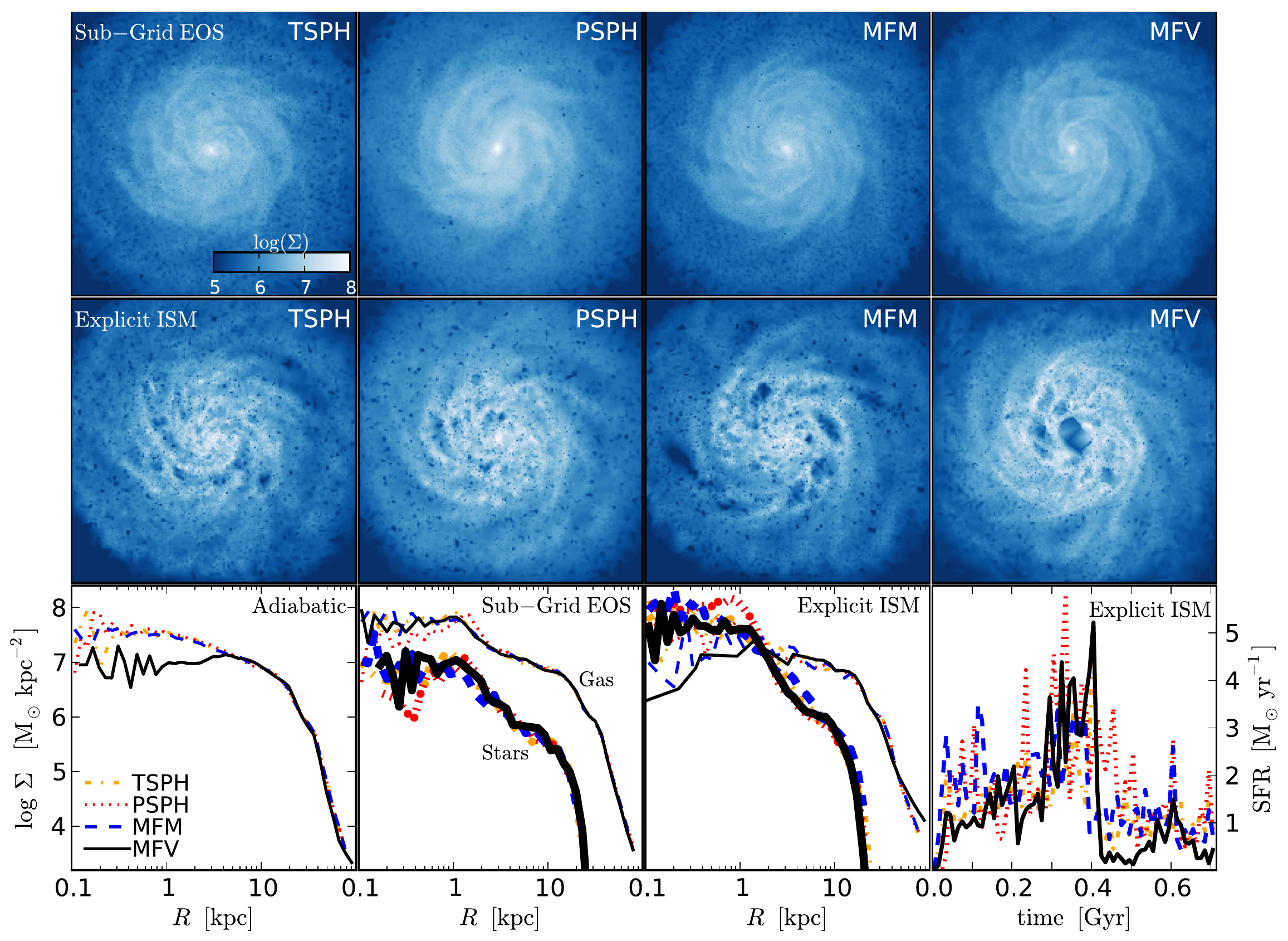
Hopkins 2015 – Traditional SPH (TSPH), Modern SPH (PSPH), Mesh-less Finite Mass (MSM), and Mesh-less Finite Volume (MFV).

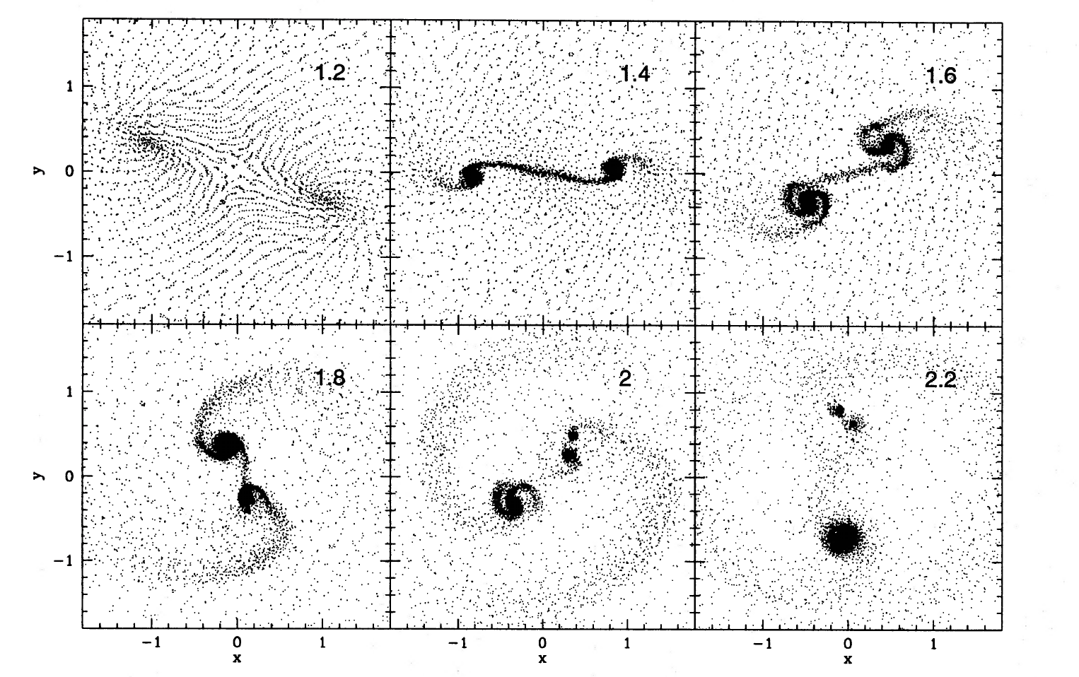
5.4 Star formation

Bate et al. (1995)

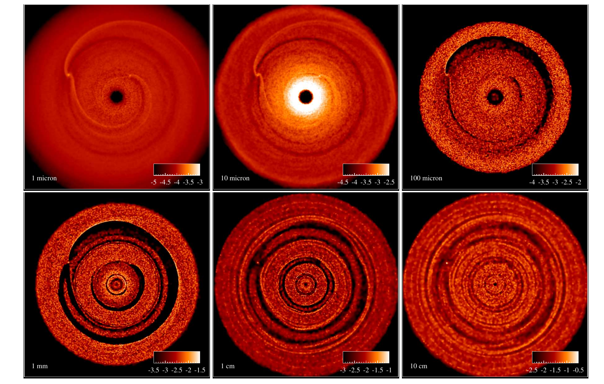
5.5 Planet formation

Dipierro et al. (2015)

5.6 Moon formation

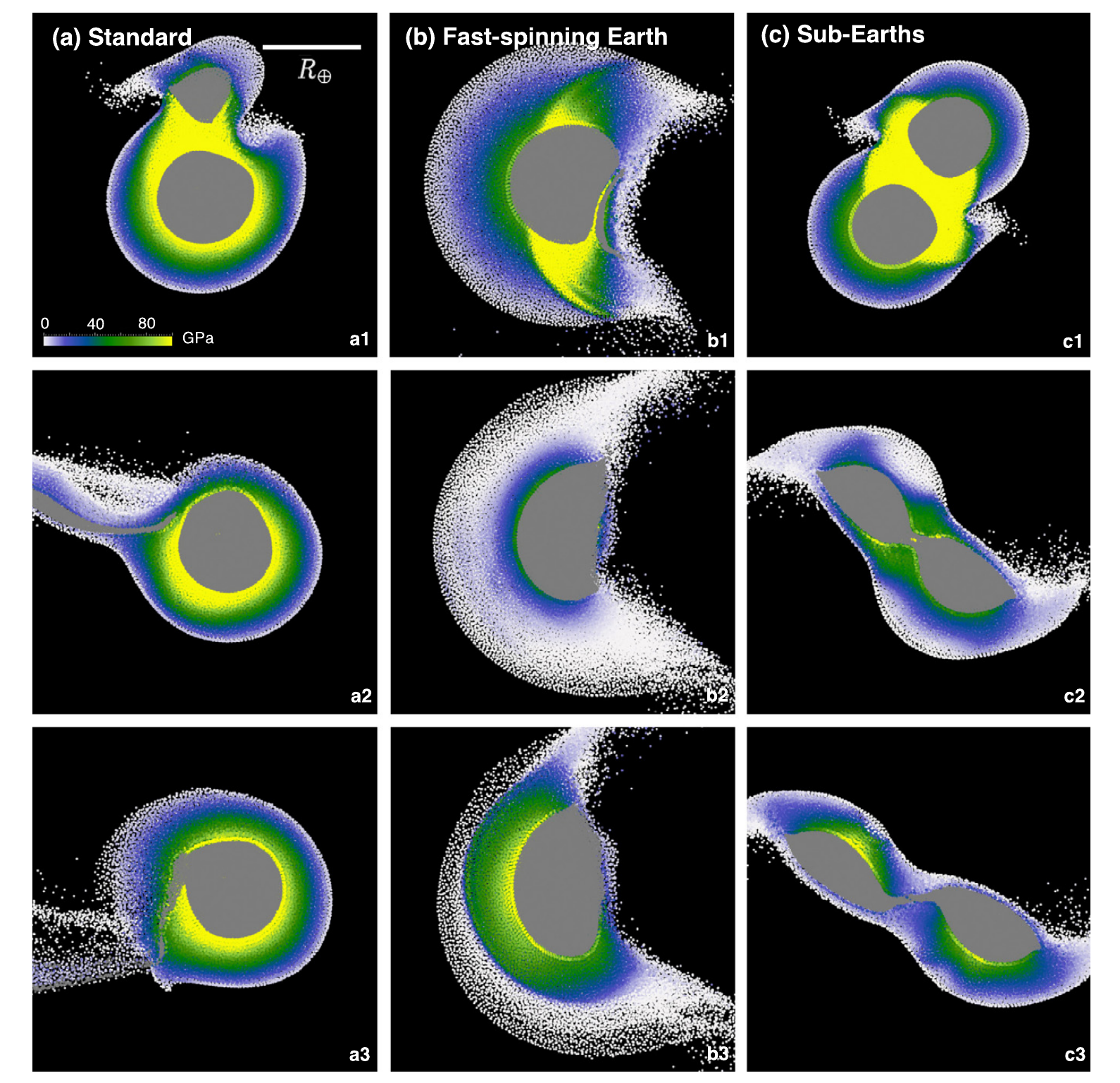
Nakajima and Stevenson (2015) (a) standard: a Mars-sized impactor hits the proto-Earth, (b) fast-spinning Earth: a small impactor hits a rapidly rotating proto-Earth, and (c) sub-Earths: two half Earth-sized planets collide.

6 Hands-on session

6.1 Hands-on session

Download the code

git clone https://github.com/pmocz/sph-python
cd sph-python

Run the code

python sph.py

Tasks:

What quantities are plotted?
Why the final curve is not the same as the theoretical prediction?
How do you interpret the particle motion?
Why the oscillation amplitudes decrease in time?
How to decrease the oscillations of particles?