Lecture 12: Hybrid and Gyrokinetic approaches – Lecture

Jan Benáček

Institute for Physics and Astronomy, University of Potsdam

January 30, 2025

1 Lecture overview

Table of Contents 1/2

17.10. Introduction + numerical methods summary
24.10. Numerical methods of differential equations — lecture + hands-on
31.10. State holiday
07.11. Test particle approach — lecture
14.11. Test particle approach — lecture + hands-on
21.11. PIC method — lecture
28.11. PIC method — hands-on

Table of Contents 2/2

05.12. Fluid and MHD — lecture (online)
12.12. Fluid and MHD — hands-on given Xin-Yue Shi
19.12. Canceled
09.01. Radiative transfer — lecture + hands-on
16.01. HPC computing — lecture + hands-on
23.01. Advanced — Smooth particle hydrodynamics method — lecture
30.01. Advanced — Hybrid, Gyrokinetics — lecture
06.02. Advanced — Vlasov and Linear Vlasov dispersion solvers — lecture

2 Introduction to hybrid codes

2.1 Introduction

In plasma physics a hybrid code refers to a model where
- Some species are treated kinetically: unknown is the distribution function \(f\), governed by the Vlasov/Boltzmann eq., solved by PIC or Vlasov methods.
- Other species are treated as a fluid: unknowns are momenta of the distribution function, governed by fluid eqs for conservation of mass, momentum, energy, etc.
In space plasma physics:
- All ion species are treated kinetically.
- Electrons are treated as a fluid.

2.2 Range of typical applicability

Range of validity of different plasma codes based on typical magnetospheric parameters: \(n=50cm^{-3}\), \(B=50 nT\), \(T_e=T_i=100 eV\) (Winske and Omidi (1996)).

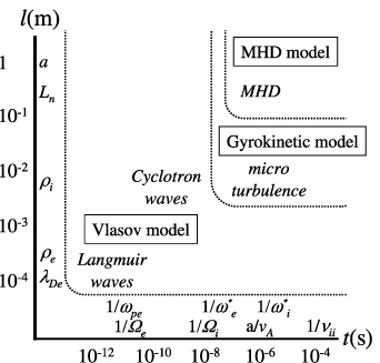
2.3 Range of typical applicability

Validity range of different plasma codes [Credits: space.aalto.fi].

3 Hybrid-kinetic equations

3.1 Hybrid-kinetic description

Hybrid-kinetic description in the Darwin limit and for \(m_e=0\)

\[ \nabla\cdot\vec{B}=0\\ \nabla\times\vec{E}=-\frac{\partial \vec{B}}{\partial t}\\ \nabla\times\vec{B}=\mu_0\vec{J}\\ \left[\frac{\partial}{\partial t} + \vec{v}\cdot\frac{\partial}{\partial \vec{x}}+\frac{q_{\alpha}}{m_{\alpha}}\left(\vec{E}+\vec{v}\times\vec{B}\right)\cdot\frac{\partial}{\partial \vec{v}}\right]f_{\alpha}=0 \\ \]

\[ \rho=\sum\limits_{\alpha} q_{\alpha}\int\limits dv^3\,f_{\alpha}\\ \vec{J}=\sum\limits_{\alpha} q_{\alpha}\int dv^3\,\vec{v}f_{\alpha} - en_e\vec{V}_e\\ 0=-en_e(\vec{E}+\vec{V}_e\times\vec{B})-\nabla P_e + en_e\eta\vec{J}\\ en_e=\sum_{\alpha}q_{\alpha}n_{\alpha}\\ P_e=T_{e0}n_e^{\gamma} \]

where \(\alpha\) are ions species.

3.2 Options for generalized Ohm’s law

Note that the electron equation of motion is a generalized Ohm’s law, which can be written in several forms: \[ 0 =-en_e(\vec{E}+\vec{V}_e\times\vec{B})-\nabla P_e + en_e\eta\vec{J}\\ \vec{E} = -\vec{V}_e\times\vec{B} - \frac{\nabla P_e}{en_e} + \eta\vec{J}\\ \vec{E} = -\vec{V}_i\times\vec{B} + \frac{\vec{J}\times\vec{B}}{en_e} - \frac{\nabla P_e}{en_e} + \eta\vec{J}\\ \vec{E} = -\vec{V}_i\times\vec{B} + \frac{(\nabla\times\vec{B}/\mu_0)\times\vec{B}}{en_e} - \frac{\nabla P_e}{en_e} + \eta\vec{J} \]

3.3 Hybrid-kinetic description

Note that the discretized Vlasov Equation is formally equivalent to the Lorentz force, \[ \frac{d\vec{v}_p}{dt}=\frac{q_p}{m_p}\left[\vec{E}_p(\vec{x},t)+\vec{v}\times\vec{B}_p(\vec{x},t)\right], \qquad(1)\] but with the EM fields defined only at the grid points and smoothed out by the shape function: \[ \vec{E}_p=\vec{E}(\vec{x}_p) = \int \vec{E}(\vec{x})S(\vec{x} -\vec{x}_p)=\sum_{\vec{x}_c}\vec{E}(\vec{x}_c)W(\vec{x}_c - \vec{x}_p)\\ \vec{B}_p=\vec{B}(\vec{x}_p) = \int \vec{B}(\vec{x})S(\vec{x} -\vec{x}_p)=\sum_{\vec{x}_c}\vec{B}(\vec{x}_c)W(\vec{x}_c - \vec{x}_p) \qquad(2)\]

\(q_p\) and \(m_p\) correspond to the charge and mass of each macroparticle (not the physical particle). The sum runs over all the cell vertices (\(\vec{x}_c\)) at the boundaries of each cell volume.

3.4 Units and spatial grid

1D ion-electron hybrid-plasma model with a background magnetic field \(\vec{B}_0(x)\).
\(\vec{E}\), \(n_i\), \(\vec{J}_i\), \(P_e\) located on the vertices of the grid, while \(\vec{B}\) is located at the center of the grid (so that curl of \(\vec{E}\) is obtained at the location of \(\vec{B}\), and curl of \(\vec{B}\) at the location of \(\vec{E}\)).
Standard normalization: ion gyrofrequency \(\Omega_{ci}\), velocity to the Alfvén speed (\(V_A\)): not constant in Maxwell eqs.
Frequency ratio \(\omega_{pi}/\Omega_{ci}=c/V_A\) is arbitrary, it can be determined by choosing density and B field in absolute units.

3.5 Resistivity

Sometimes an effective resistivity \(\eta\) is added, which represents wave-particle effects due to high-frequency waves \(\omega>\Omega_{ci}\) (Matsumoto and Omura (1993)).
In practice, an “anomalous” electron-ion collision frequency \(\nu_{an}\) is added, related to the resistivity \[ \eta=\frac{\nu_{an}}{\epsilon_0\omega_{pe}^2} \]
The effective value of \(\eta\) is chosen in terms of the associated resistive length \[ L_{\eta}= \frac{\eta}{\mu_0 V}= \frac{\nu_{an}c^2}{\omega_{pe}^2 V} \] where usually \(L_{\eta}<0.1\Delta x\).
This is specially used to eliminate high frequency noise (e.g.: in some shock problems), where \(\nu_{an}\) corresponds to the collision frequency associated to the lower-hybrid frequency, consistent with cross-field instabilities.

3.6 Approaches to bring both approaches together

The most popular hybrid-kinetic plasma model applied to space physics considers the following approximations
- Darwin approximation for EM fields. No displacement current in Ampére’s equation (no retarded potentials), magneto-inductive model, no electromagnetic waves.
- Electrons with zero mass, i.e., from the electron momentum equation: \[ 0=-en_e(\vec{E}+\vec{V}_e\times\vec{B})-\nabla P_e + en_e\eta\vec{J} \]
- Adiabatic equation of state, scalar pressure.
- Charge (quasi)-neutrality.

4 Applications

4.1 Normal plasma modes

4.2 Numerical dispersion relation

How to numerically determine a wave dispersion relation using the output of a PIC code? 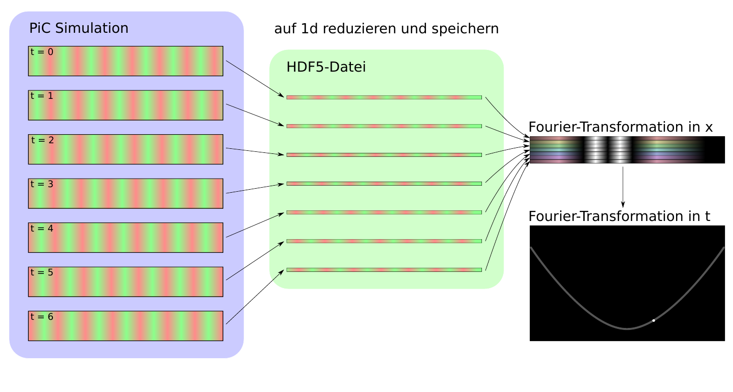Real EM dispersion relation

4.3 Normal plasma modes

Transverse modes

4.4 Normal plasma modes

Electrostatic perpendicular modes .

4.5 Beam instabilities

4.6 1D Ion beam instabilities

Weak ion beam (i.e.: density \(n_b\ll n_0\)) propagating on an background ion population
\(n_0=n_b + n_i\) (both ions species = protons here).
Ion beam drifting \(V_B\gg V_A\) along an uniform \(B_0\).
Charge neutralizing electron background at rest.
No net current: \[ V_b' = ( 1 - n_b/n_0)V_b\\ V_i' = - (n_b/n_0)V_b \]
The solution of the linear dispersion relation (assuming \(\omega=\omega_r+i\gamma\)) predicts instability (\(\gamma>0\)) if: \[ \omega - k V_b + \Omega_{ci} = 0 \] i.e.: beam ions are in cyclotron resonance with the waves. In the beam reference frame waves are L-handed polarized (ion-cyclotron), while in the electron frame they are R-handed polarized.
\(\gamma\) increases with \(n_b/n_0\).
In the examples here, \(V_B=10V_A\), \(\beta_i=1\), \(n_b/n_0=0.015\) (Matsumoto and Omura (1993)).

4.7 1D Ion beam instability

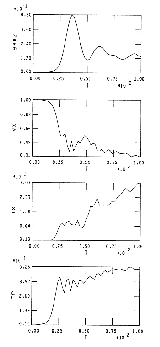
Energies .

4.8 1D Ion beam instability

\(t=20\Omega_{ci}^{-1}\) .

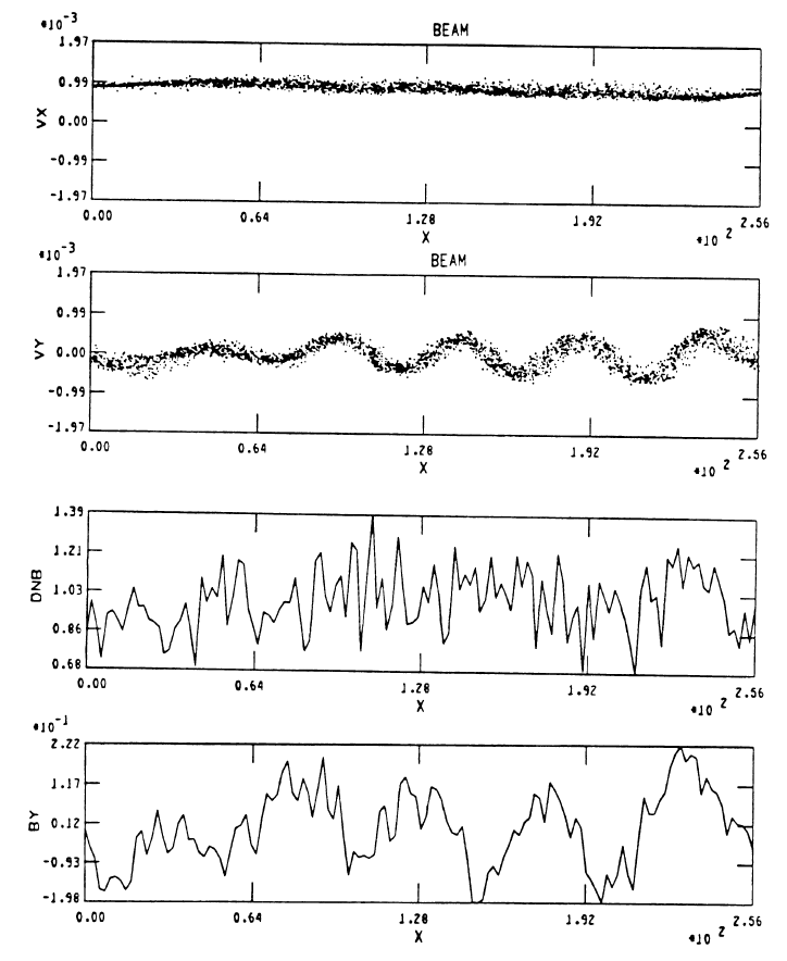
4.9 1D Ion beam instability

\(t=40\Omega_{ci}^{-1}\) .

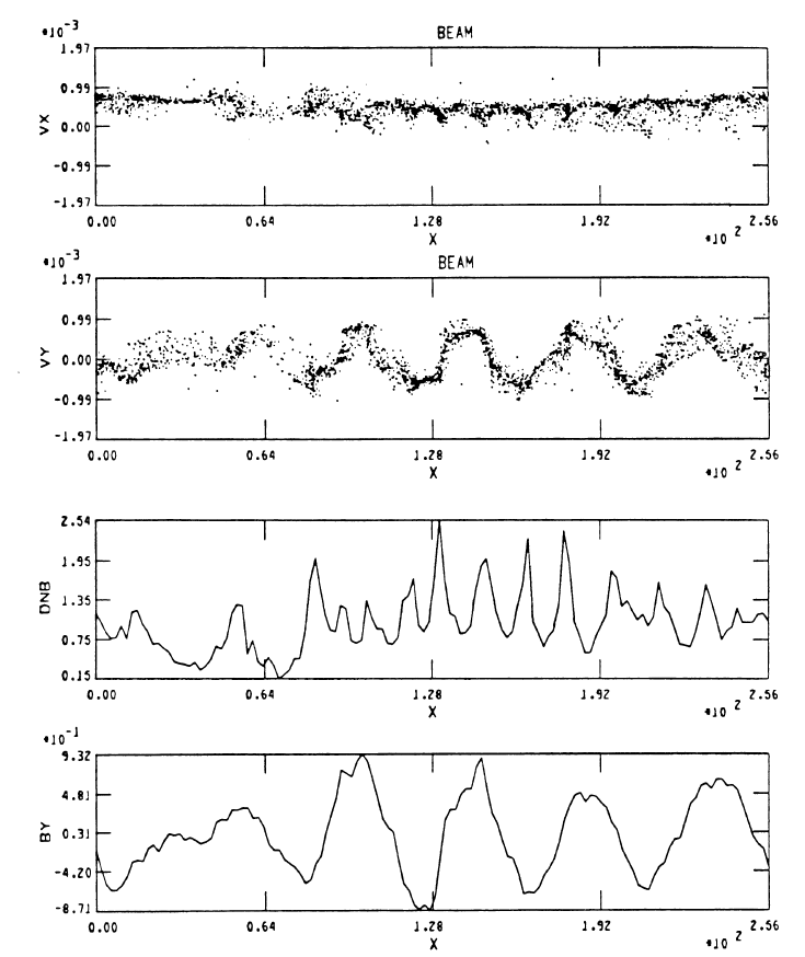
4.10 1D Ion beam instability

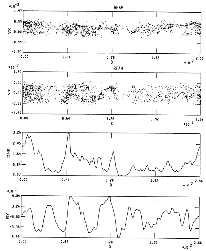
\(t=60\Omega_{ci}^{-1}\) .

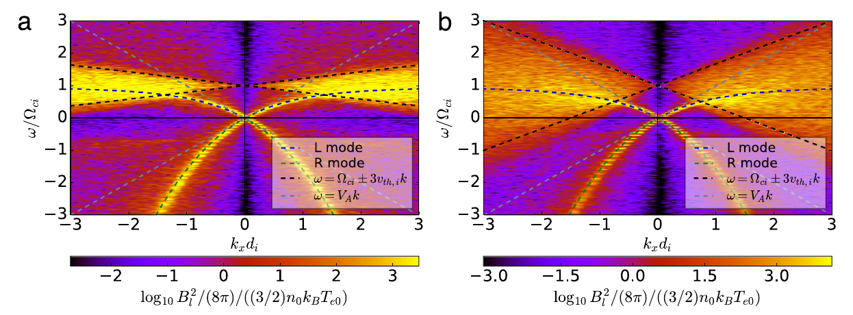
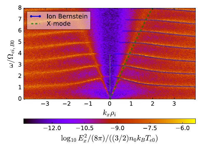
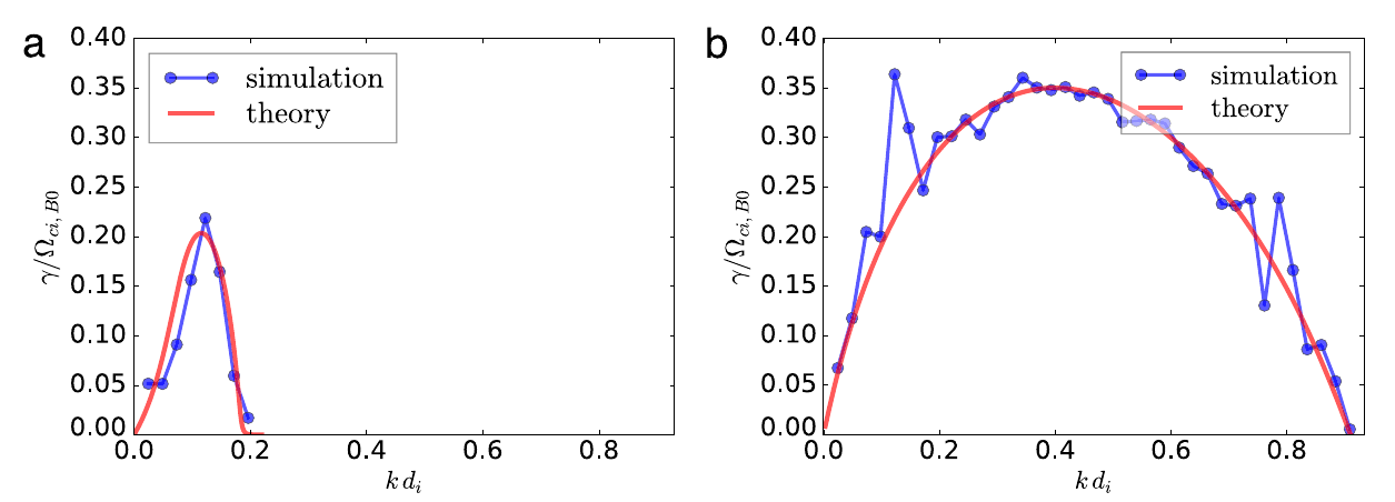
4.11 1D Ion beam instability

Numerical dispersion relation .

4.12 1D Ion beam instability

Time evolution of Fourier modes .

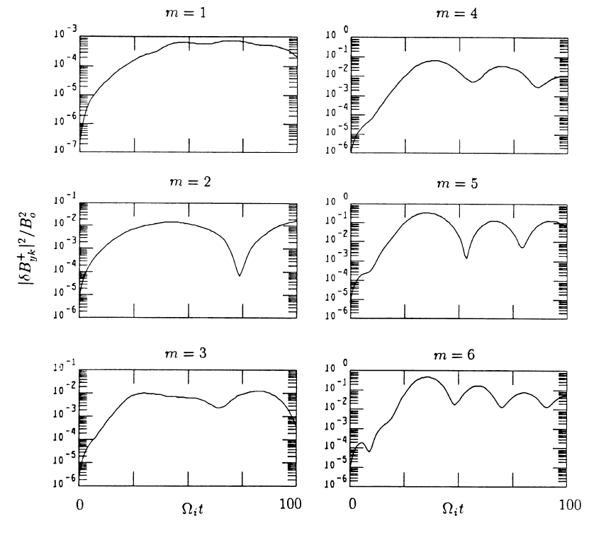
4.13 1D Ion beam instability

Comparison of growth rates: simulation/theory (Muñoz et al. (2018))

4.14 Magnetic reconnection

4.15 Magnetic reconnection

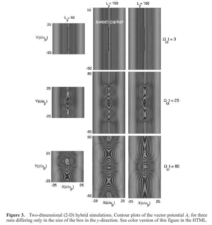
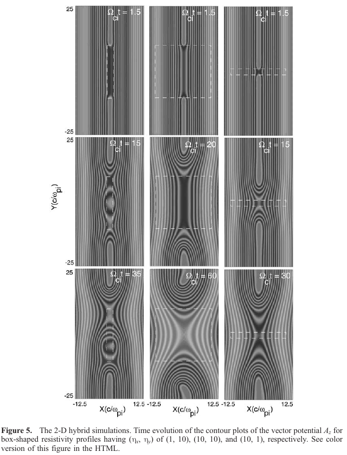
4.16 Magnetic reconnection: resistivity effects

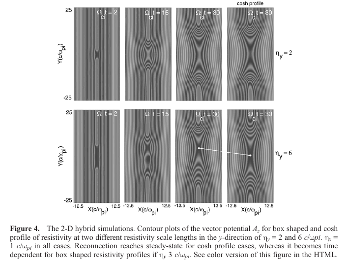
4.17 Magnetic reconnection: resistivity effects

5 Gyrokinetic approach

5.1 Notation

Cyclotron frequency of species \(\alpha\) are denote by capital \(\Omega_{c \alpha}\),
Typical size of the problem is \(l_0\),
\(\rho_i\) is not density or charge density, but the Larmor gyro-radius,
Quantities \(f\), \(F\), and \(h_s\) denote velocity distributions in various interpretations.
Often used quantity \(k_\parallel \rho_i\) (\(k_\perp \rho_i\)) can interpreted as \[ \sim 2\pi\frac{\rho_i}{\lambda} \sim \frac{\rho_i}{\lambda} \]
For longer wavelengths that the Larmor gyro-radius, \(\lambda \gg \rho_i,\) and \(k_\parallel \rho_i \rightarrow 0\).

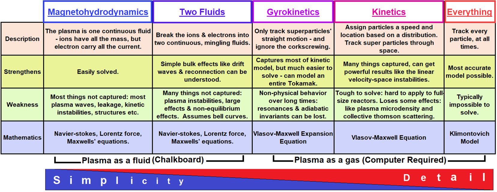
5.2 Introduction

Vlasov equation is 6D: \(f(\vec{x}, \vec{v};t)\)
The gyromotion of particles can be neglected when, e.g., the plasma is strongly magnetized.
This implies that only the gyrocenter/guiding center of the particles is tracked, and the dimensionality of the problem is 5D: \(f(\vec{X}, v_{\parallel}, \mu;t)\), making it computationally less demanding (\(\mu\) is the magnetic moment)

Gyrokinetics transformation

5.3 Introduction

Schematics of gyrokinetics

5.4 Introduction

Schematics of gyrokinetics

5.5 Assumptions of the gyrokinetic (GK) model

Strongly magnetized conditions:

Larmor radius: \[ \rho_i=\frac{v_{th,i}}{\Omega_{ci}}\ll l_0 \] where \(l_0\) is a typical gradient length scale; below denoted as the typical parallel wavelength of the fluctuations.

This defines the ordering/expansion parameter \(\epsilon\) \[ \epsilon=\frac{\rho_i}{l_0}\ll 1 \]

Low frequency phenomena: \[ \omega \sim \frac{v_{th,i}}{l_0}\sim \mathcal{O}(\epsilon \Omega_{ci})\ll\Omega_{ci} \] this allows to average over the particles’ gyroradii.

5.6 Assumptions of the gyrokinetic (GK) model

Small fluctuations with respect to the equilibrium:

Let \(F_0\), \(B_0\) and \(E_0=v_{th, i}B_0\) be the equilibrium distribution function and \(\delta f_1\), \(\delta \vec{B}\), and \(\delta \vec{E}\) are their perturbations.

Then, we have, \[ \frac{\delta f_1}{F_0} \sim \frac{\delta \vec{B}}{B_0} \sim \frac{\delta \vec{E}}{v_{th, i}B_0}\sim\mathcal{O}(\epsilon ) \qquad(3)\]

The equilibrium distribution function is allowed to vary slow enough: \[ \frac{1}{F_0}\frac{\partial F_0}{\partial t}\sim \mathcal{O}\left(\frac{1}{t_{\rm heat}}\right). \] where \(t_{\rm heat}\) is the so called heating time-scale: \[ t_{\rm heat} = \frac{1}{\epsilon^2}\frac{l_0}{v_{th, i}}\sim\mathcal{O}\left(\frac{1}{\epsilon^3\Omega_{ci}}\right) \]

5.7 Assumptions of the gyrokinetic (GK) model

Small/large spatial fluctuations across/along the magnetic field. \[ k_{\perp} \sim \frac{\hat{b}\times\nabla \delta f}{\delta f} \sim \frac{\hat{b}\times\nabla \delta \vec{B}}{|\delta \vec{B}|} \sim \frac{\hat{b}\times\nabla \delta \vec{E}}{|\delta \vec{E}|}\sim \mathcal{O}\left(\frac{1}{\rho_i}\right)\qquad \Leftrightarrow\qquad k_{\perp}\rho_i\sim 1\\ k_{\parallel} \sim \frac{\hat{b}\cdot\nabla \delta f_1}{\delta f} \sim \frac{\hat{b}\cdot\nabla \delta \vec{B}}{|\delta \vec{B}|} \sim \frac{\hat{b}\cdot\nabla \delta \vec{E}}{|\delta \vec{E}|}\sim \mathcal{O}\left(\frac{1}{l_0}\right) \]

where \(\hat{b}=\vec{B}_0/B_0\)
Then, the anisotropy of the fluctuations is \[ \frac{k_{\parallel}}{k_{\perp}} = \frac{\rho_i}{l_0}\sim\mathcal{O}\left(\frac{\rho_i}{l_0}\right)\sim\mathcal{O}(\epsilon) \ll 1, \qquad(4)\]

which agrees with a key prediction of MHD turbulence as well as solar wind observations.

5.8 Assumptions of the gyrokinetic (GK) model

The relation between \(k_{\parallel}\) and \(k_{\perp}\) also constrains \(V_{\perp}\).

Since the dominant drift tends to be \(\vec{E}\times\vec{B}\), we have: \[ \vec{V}_{\perp} \sim \frac{\delta\vec{E}\times \vec{B}_0}{B_0^2} \sim \mathcal{O}(\epsilon v_{th, i}) \qquad(5)\]

Thus, the maximum spatial fluctuations perpendicular to the magnetic field are of order \[ L_{\perp} \sim \frac{|\vec{V}_{\perp}|}{\omega} \sim \frac{1}{k_{\perp}} \sim \mathcal{O}(\rho_i) \]

No restriction on \(\beta\), \(k_{\perp}\rho\), \(\omega/(k_{\parallel}v_{th})\), \(\omega/\nu\)
Note that there are 3 time scales:

\(\Omega_{ci}^{-1}\) (fast, upper limit), \(\omega^{-1}\) (typical GK wave frequencies), \(t_{heat}\) (slow, lower limit)

5.9 Consequences of the assumptions of the GK model

All cyclotron-frequency effects (cyclotron resonances), fast MHD waves and high-frequency kinetic waves (e.g.; Langmuir) are ordered out \(\Rightarrow\) Computational savings of order of magnitude compared to fully kinetic models.
Slow MHD and Alfvén MHD waves are retained.
In general, all kinetic effects for low frequency micro-turbulence are maintained.
Collisionless dissipation occurs via Landau damping or similar mechanisms.

5.10 Parallel/Perpendicular fluctuations

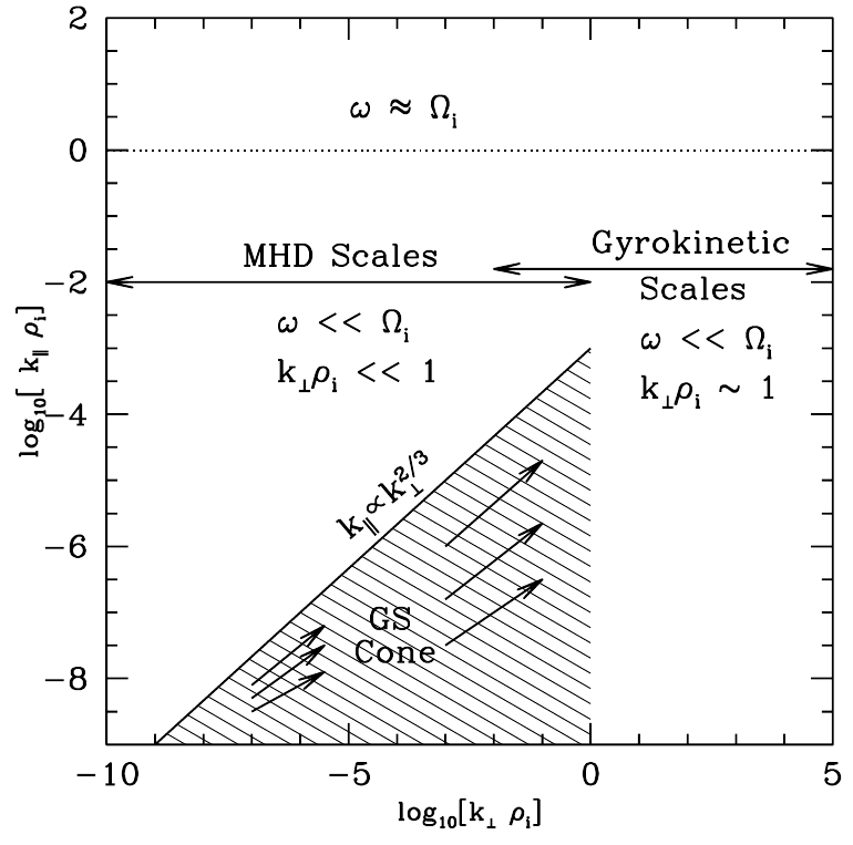
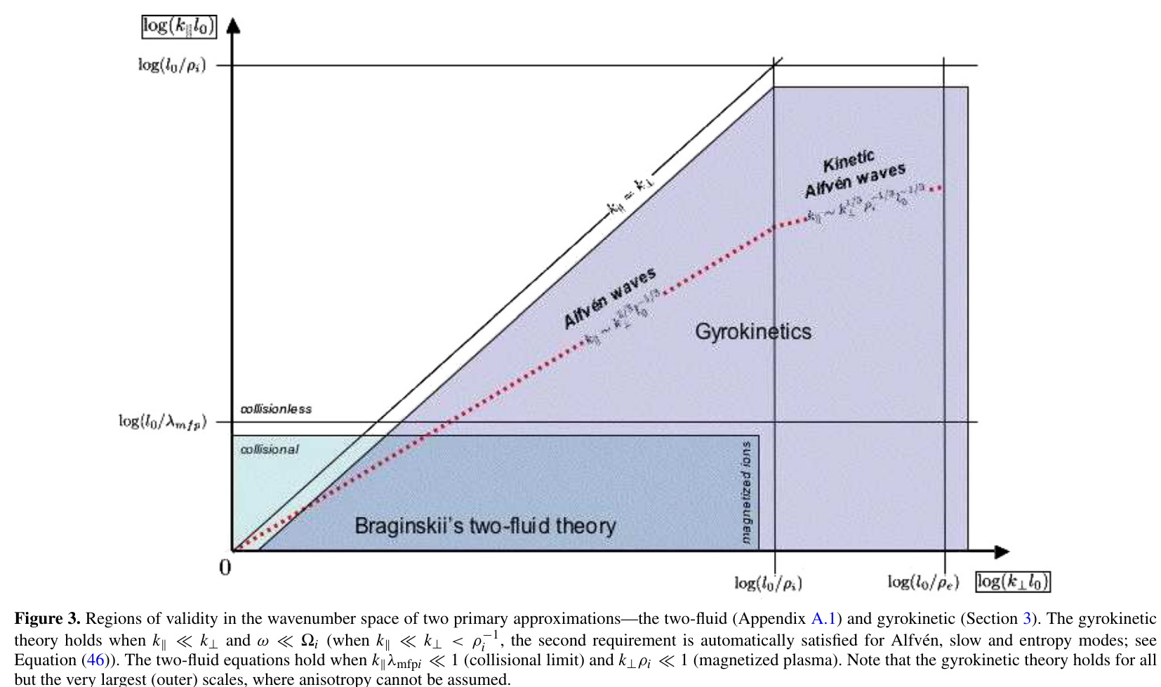
Range of validity of GK (Gregory G. Howes et al. (2006)).

6 Gyrokinetic equations

6.1 Coordinates and averages

Guiding center coordinates and particle velocity decomposition \[ \vec{r} = \vec{R_s} - \frac{\vec{v}\times\hat{z}}{\Omega_s}\\ \vec{v} = v_{\parallel} \hat{z} + v_{\perp} (\cos\theta\hat{x} + \sin\theta\hat{y}) \] where the guiding center is \(\vec{R}_s\) and the instantaneous particle’s position is \(\vec{r}\). The background magnetic field is along \(\hat{z}\).

6.2 Coordinates and averages

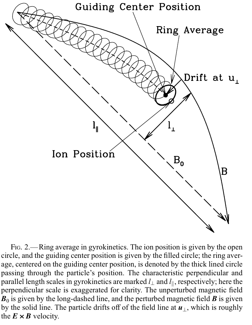
(Gregory G. Howes et al. (2006))

6.3 Coordinates and averages

GK averages of any function \(a(\vec{r},\vec{v},t)\) over the Larmor radius, at fixed guiding center \(\vec{R}_s\) and fixed position \(\vec{r}\), respectively Gregory G. Howes et al. (2006) \[ \langle a(\vec{r},\vec{v},t)\rangle_{\vec{R}_s} = \frac{1}{2\pi}\oint d\theta a\left( \vec{R}_s - \frac{\vec{v}\times\hat{z}}{\Omega_s},\vec{v},t\right)\\ \langle a(\vec{R}_s,\vec{v},t)\rangle_{\vec{R}_s} = \frac{1}{2\pi}\oint d\theta a\left( \vec{r} + \frac{\vec{v}\times\hat{z}}{\Omega_s},\vec{v},t\right) \] where both averages are also at constant \(v_{\parallel}\) and \(v_{\perp}\).

6.4 Pop-culture reference of gyrokinetics

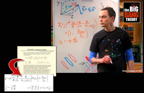
The Big Bang Theory and gyrokinetics.

6.5 Gyrokinetic equation

Expansion of the full plasma distribution function: \[ f_s = F_{0s}(v,t)\exp\left(-\frac{q_s\phi(\vec{r},t)}{T_{0s}}\right) + h_s(\vec{R}_s,v,v_{\perp},t)+ \delta f_{2s} \] where \(\exp\left(-\frac{q_s\phi(\vec{r},t)}{T_{0s}}\right)\) is the Boltzmann factor, the equilibrium distribution function is a Maxwellian \[ F_{0s} = \frac{n_{0s}}{\pi^{3/2}v_{th,s}^3}\exp\left(\frac{-v^2}{v_{th,s}^2}\right) \] and \(h_s(\vec{R}_s,v,v_{\perp},t)\) is the gyrokinetic/ring-averaged distribution function of the guiding center.
Other formulations use the kinetic energy \(K=m_sv^2/2\) and the first adiabatic invariant (magnetic moment) \(\mu_s = \frac{1}{2}m_s v_{\perp}^2/B_0\) instead of \(v\) and \(v_{\perp}\), respectively. \(\mu_s\) can also be replaced by the pitch angle \(\lambda = \mu_s/K\).

6.6 Gyrokinetic equation

The ring distribution \(h_s\) satisfies the gyrokinetic equation (Frieman and Chen (1982),Gregory G. Howes et al. (2006),Schekochihin et al. (2009),Brizard and Hahm (2007),Catto (2019)) \[ \frac{\partial h_s}{\partial t} + v_{\parallel}\hat{b}\cdot\frac{\partial h_s}{\partial \vec{R}_s} + \frac{c}{B_0}\left[ \langle \chi\rangle_{\vec{R}_s}, h_s\right] -\left(\frac{\partial h_s}{\partial t}\right)_{coll} = q_s\frac{\partial \langle \chi\rangle_{\vec{R}_s}}{\partial t}\frac{F_{0s}}{T_{0s}} \qquad(6)\] where the gyrokinetic potential \(\chi\) is expressed in terms of the standard EM potentials: \[ \chi =\phi - \vec{v}\cdot\vec{A}/c\\ \vec{E} =-\nabla\phi - (1/c)\partial\vec{A}/\partial t\\ \vec{B} = \nabla\times\vec{A} \] and the Poisson brackets are: \[ [U,V]=\hat{b}\cdot\left(\frac{\partial U}{\partial \vec{R}_s}\times\frac{\partial V}{\partial \vec{R}_s}\right) \]

6.7 Gyrokinetic equation

\[ \frac{\partial h_s}{\partial t} + v_{\parallel}\hat{b}\cdot\frac{\partial h_s}{\partial \vec{R}_s} + \frac{c}{B_0}\left[ \langle \chi\rangle_{\vec{R}_s}, h_s\right] -\left(\frac{\partial h_s}{\partial t}\right)_{coll} = q_s\frac{\partial \langle \chi\rangle_{\vec{R}_s}}{\partial t}\frac{F_{0s}}{T_{0s}} \] can be compared with Vlasov–Boltzman equation without gyrokinetic approximation. \[ \frac{\partial f_{\alpha}}{\partial t} + \vec{v}\cdot\frac{\partial f_{\alpha}}{\partial \vec{x}}+\frac{q_{\alpha}}{m_{\alpha}}\left(\vec{E}(\vec{x},t)+\vec{v}\times\vec{B}(\vec{x},t)\right)\cdot\frac{\partial f_{\alpha}}{\partial \vec{v}}= \left( \frac{\partial f_\alpha}{\partial t} \right)_{coll} \qquad(7)\]

6.8 Gyrokinetic equation

Another form of the gyrokinetic equation Equation 6 is: \[ \frac{\partial h_s}{\partial t} + \left\langle \frac{d\vec{R}_s}{dt} \right\rangle_{\vec{R}_s}\cdot\frac{\partial h_s}{\partial \vec{R}_s} - \left(\frac{\partial h_s}{\partial t}\right)_{\rm coll} = \left\langle \frac{d\mathcal{E}_s}{dt} \right\rangle_{\vec{R}_s}\frac{F_{0s}}{T_{0s}} \qquad(8)\] where \(\mathcal{E}_s=\frac{1}{2}m_sv^2 + q\phi\) is the total energy of the particle.

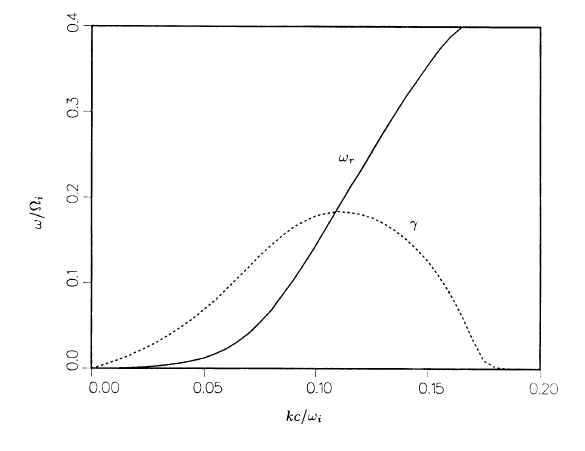
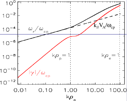
6.9 Limits of applicability of GK

GK theory breaks down when these conditions are not satisfied: \(k_{\parallel}\ll k_{\perp}\), \(\omega\ll\Omega_{ci}\), \(v_{th,i}\ll c\), so in the plot below both GK \(\gamma\) and \(\omega\) deviate from the full Vlasov solutions when the first two conditions are not met.

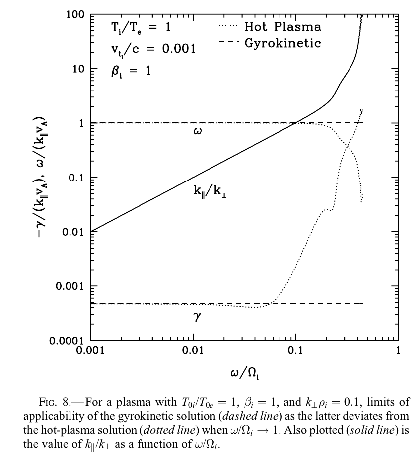
Gregory G. Howes et al. (2006)

7 Numerical approaches of Gyrokinetics

7.1 Numerical considerations

The GK eqs. continuosly produces fine scale velocity space structures via the ballistic term, leading to fine scale structures in \(v_{\parallel}\): filamentation (see our lecture next week).
Driven turbulence (by, e.g., an antenna), because homogeneous turbulence is always damped. Energy input from the antenna is dissipated by heating the plasma species.
There are three types of numerical methods (Garbet et al. (2010)):

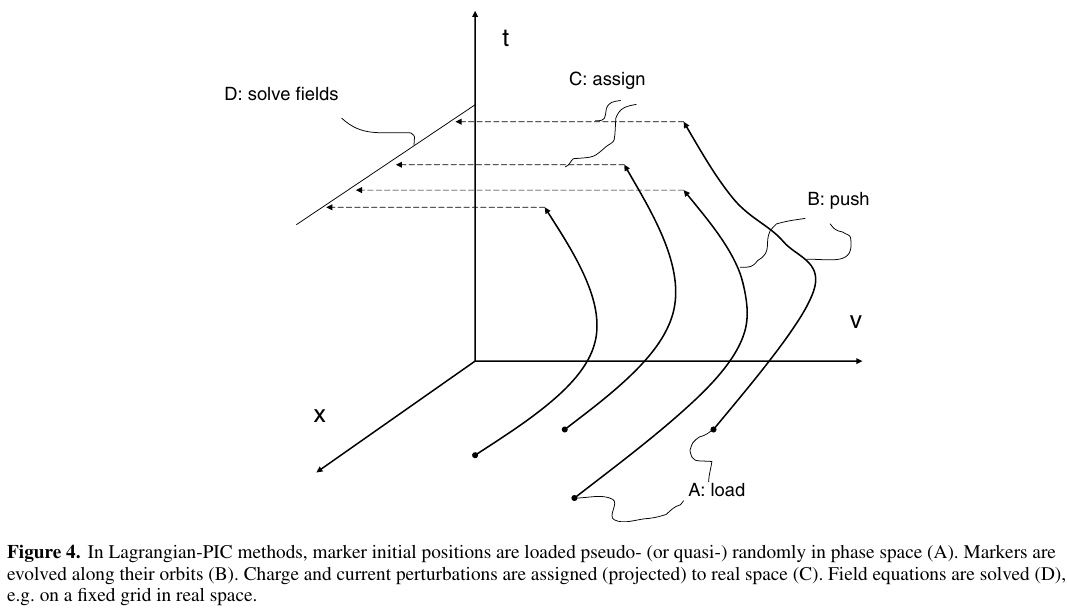
7.2 1. GK Lagrangian/PIC approach

7.3 1. GK Lagrangian/PIC approach

First numerical approach for gyrokinetics in the 80s
Based on the Liouville’s theorem for the ring (gyrocenter) distribution, sampled by macroparticles.
It is numerically cheap and very suitable for HPC computing.
But the method is noisy due to its statistical nature.

This is the reason why most of the PIC-GK codes advance only the fluctuating distribution function (\(\delta f\) method), so that the noise is reduced.

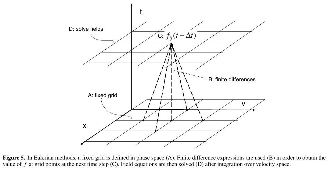
7.4 2. GK Eulerian/Vlasov approach

Range of validity of GK Gregory G. Howes et al. (2006).

7.5 2. GK Eulerian/Vlasov approach

Toward the late 1990s, first attempts to explore a gid-based (Eulerian) approach to solve the GK equations (GENE Jenko et al. (2000), GS2 Dorland et al. (2000)} \(\rightarrow\) AstroGK Numata et al. (2010) codes)
Discretization of the gyrocenter distribution function in the full 5D space
Equations are solved by using a mix of either finite differences, finite volumes, finite element methods or spectral Fourier (standard CFD methods) in space, and time-explicit higher-order (e.g.: Runge-Kutta) or implicit schemes in time.
Computationally competitive compared to PIC approaches, noise is absent, but issues with numerical dissipation/overshoot (too little or too much), positivity of the distribution function

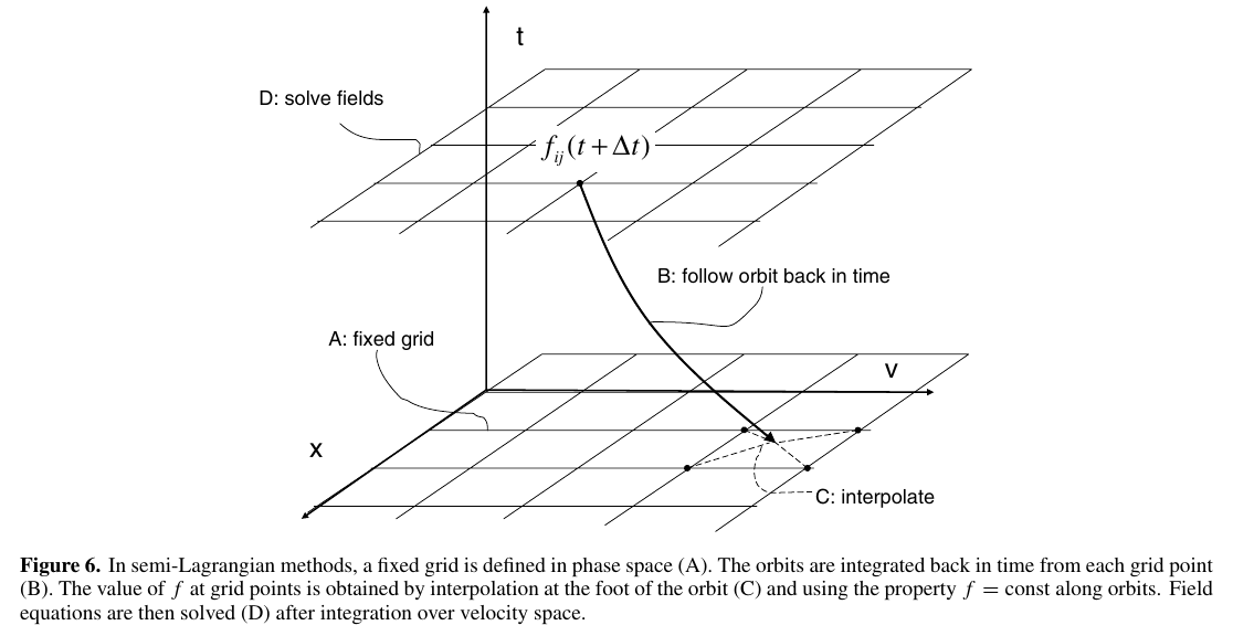
7.6 3. GK Semi-Lagrangian approach

Range of validity of GK Gregory G. Howes et al. (2006).

8 Applications

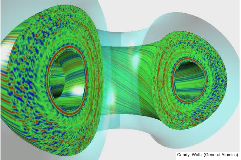
8.1 Fusion devices: Tokamaks

Turbulence, transport in tokamaks and stellarators, driven, e.g. by temperature gradients.

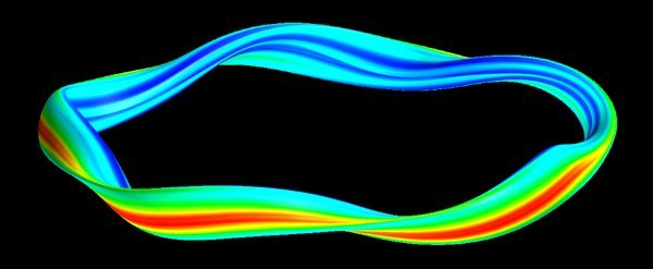
8.2 Fusion devices: Stellarators

8.3 Turbulence theory

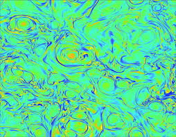
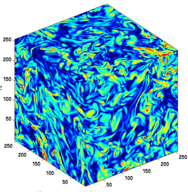
8.4 Turbulence examples

Thesis by David Thomos, 2018

8.5 Modern theory of MHD turbulence

The first fluid turbulence theory was developed by Kolmogorov in 1941. It predicts a kinetic energy scaling of \(k^{-5/3}\), matching relatively well with observations.
An extension of this theory for magnetized plasmas (MHD) was developed by Iroshnikov and Kraichnan in 1963. It predicts a \(k^{-3/2}\) at inertial scales, which failed to agree with observations.
The modern theory of MHD turbulence is based on
- It is assumed that \(k_{\parallel}\ll k_{\perp}\).
- Critical balance conjecture: times scales of linear fluctuations of Alfvén waves should be similar to the time scale of cascade of energy: \[ \omega=k_{\parallel}V_A \sim \omega_{nl}\approx k_{\perp}V_{1,\perp} \] resulting in a turbulent spectrum: \[ k_{\perp}^{-5/3}\;\;\;\text{and}\;\;\;k_{\parallel}^{-2} \qquad(9)\]

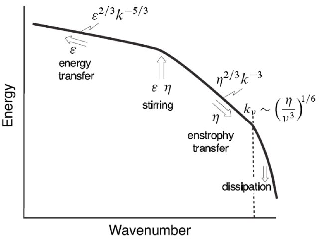
8.6 Modern theory of MHD turbulence

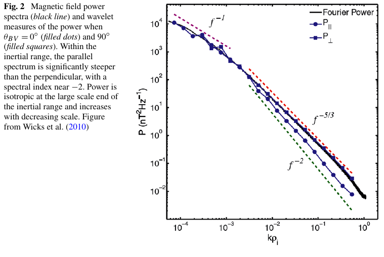
The anisotropic turbulence spectrum equation Equation 9 is often observed in solar wind, magnetosheath, ISM turbulence and MHD simulations.

8.7 MHD turbulence and gyrokinetics

The GS95 MHD turbulence theory applies to Alfvénic fluctuations, where \(\delta B_{\perp} \sim V_{\perp}\sqrt{\mu n m_i}\) (other MHD modes, like slow modes, are advected by the Alfvénic component)
Alfvén waves are damped at the ion gyroscale, while fast and slow modes at the mean free path (very large for astrophysical plasmas)
Gyrokinetic turbulence also uses the same basic assumptions of the GS 95 turbulence model, but where the basic component are Kinetic Alfvén waves, with \(\omega\sim k_{\parallel}V_A\ll \Omega_{ci}\) and simultaneously \(k_{\perp}\rho_i\sim1\) (other high frequency waves, such as whistlers, are absent).

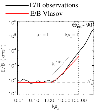
8.8 Kinetic Alfvén waves

Can be viewed as a coupling of the ion acoustic mode and the Alfvén wave, with \(k_{\parallel}\ll k_{\perp}\)
Undergo both electron and ion Landau damping, but only at scales close to \(\rho_i\).
Are associated to compressive parallel \(\vec{B}\) field fluctuations with a parallel \(\vec{E}\) component. \[ \omega_r=k_{\parallel}V_{A}k_{\perp}\rho_i/\sqrt{\beta_i + 2/(1+T_e/T_i)} \] Sahraoui et al. (2009)

8.9 Kinetic Alfvén waves and gyrokinetics

8.10 Applications to solar wind turbulence

G. G. Howes et al. (2008) carried out Eulerian GK simulations of solar wind turbulence, resulting in a turbulent spectrum being consistent with MHD simulations at \(k_{\perp}\rho_i\sim 0.1-1\) (\(k^{-5/3}\)) and a break at ion scales \(k_{\perp}\rho_i>1\) with spectral slopes matching the predictions of critically balanced turbulence. This is consistent with in-situ turbulence measurements

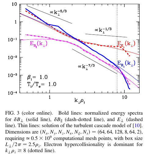
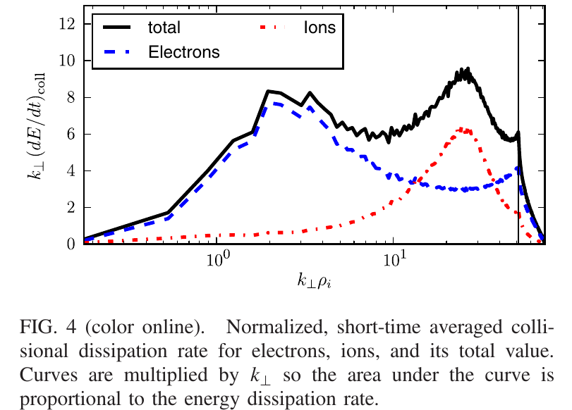
8.11 Applications to solar wind turbulence

Told et al. (2015) carried out one of the largest GK simulations of solar wind turbulence so far, covering the range \(k_{\perp}\rho_i\sim0.2-50\) including the physics at the spectral break. The scaling was consistent with critically balanced turbulence of kinetic Alfv'en waves.

8.12 From the Wikipedia article: “Gyrokinetics”

GS2: A numerical continuum code for the study of turbulence in nuclear fusion plasmas.
AstroGK: A code based on GS2 (above) for studying turbulence in astrophysical plasmas.
GENE: A semi-global continuum turbulence simulation code, for fusion (and since recently also space) plasmas.
GEM: A particle in cell turbulence code, for fusion plasmas.
GKW: A semi-global continuum gyrokinetic code, for turbulence in fusion plasmas.
GYSELA: A semi-Lagrangian code, for turbulence in fusion plasmas.
ELMFIRE: Particle in cell Monte-Carlo code, for fusion plasmas.
ORB5: Global particle in cell code, for electromagnetic turbulence in fusion plasmas.

8.13 References

Brizard, A. J., and T. S. Hahm. 2007. “Foundations of nonlinear gyrokinetic theory.” Rev. Mod. Phys. 79 (June): 421–68. https://doi.org/10.1103/RevModPhys.79.421.

Catto, Peter J. 2019. “Practical gyrokinetics.” J. Plasma Phys. 85 (3). https://doi.org/10.1017/S002237781900031X.

Dorland, William, F Jenko, M Kotschenreuther, and B. Rogers. 2000. “Electron Temperature Gradient Turbulence.” Phys. Rev. Lett. 85 (26): 5579–82. https://doi.org/10.1103/PhysRevLett.85.5579.

Frieman, E A, and Liu Chen. 1982. “Nonlinear gyrokinetic equations for low-frequency electromagnetic waves in general plasma equilibria.” Phys. Fluids 25 (1982): 502–8. https://doi.org/10.1063/1.863762.

Garbet, X., Y. Idomura, L. Villard, and T. H. Watanabe. 2010. “Gyrokinetic simulations of turbulent transport.” Nucl. Fusion 50 (4): 043002. https://doi.org/10.1088/0029-5515/50/4/043002.

Horbury, T. S., R. T. Wicks, and C. H. K. Chen. 2012. “Anisotropy in Space Plasma Turbulence: Solar Wind Observations.” Space Sci. Rev. 172 (1-4): 325–42. https://doi.org/10.1007/s11214-011-9821-9.

Howes, G. G., W. Dorland, S. C. Cowley, G. W. Hammett, E. Quataert, A. A. Schekochihin, and T. Tatsuno. 2008. “Kinetic Simulations of Magnetized Turbulence in Astrophysical Plasmas.” Phys. Rev. Lett. 100 (6): 065004. https://doi.org/10.1103/PhysRevLett.100.065004.

Howes, Gregory G., Steven C. Cowley, William Dorland, Gregory W. Hammett, Eliot Quataert, and Alexander a. Schekochihin. 2006. “Astrophysical Gyrokinetics: Basic Equations and Linear Theory.” Astrophys. J. 651 (1): 590–614. https://doi.org/10.1086/506172.

Jenko, Frank, William Dorland, M Kotschenreuther, and B N Rogers. 2000. “Electron temperature gradient driven turbulence.” Phys. Plasmas 7 (5): 1904. https://doi.org/10.1063/1.874014.

Matsumoto, H, and Y Omura. 1993. Computer Space Plasma Physics : Simulation Techniques and Software. Terra Scientific Publishing Company. https://www.terrapub.co.jp/e-library/cspp/.

Muñoz, P. A., N. Jain, P. Kilian, and J. Büchner. 2018. “A new hybrid code (CHIEF) implementing the inertial electron fluid equation without approximation.” Computer Physics Communications 224 (March): 245–64. https://doi.org/10.1016/j.cpc.2017.10.012.

Numata, Ryusuke, Gregory G. Howes, Tomoya Tatsuno, Michael Barnes, and William Dorland. 2010. “AstroGK: Astrophysical gyrokinetics code.” J. Comput. Phys. 229 (24): 9347–72. https://doi.org/10.1016/j.jcp.2010.09.006.

Sahraoui, F., M. L. Goldstein, P. Robert, and Yu V. Khotyaintsev. 2009. “Evidence of a Cascade and Dissipation of Solar-Wind Turbulence at the Electron Gyroscale.” Phys. Rev. Lett. 102 (23): 231102. https://doi.org/10.1103/PhysRevLett.102.231102.

Schekochihin, Alexander A., S. C. Cowley, William Dorland, G W Hammett, Gregory G. Howes, E Quataert, and T Tatsuno. 2009. “Astrophysical Gyrokinetics: Kinetic and Fluid Turbulent Cascades in Magnetized Weakly Collisional Plasmas.” Astrophys. J. Suppl. Ser. 182 (1): 310–77. https://doi.org/10.1088/0067-0049/182/1/310.

Told, D., F. Jenko, J. M. TenBarge, G. G. Howes, and G. W. Hammett. 2015. “Multiscale Nature of the Dissipation Range in Gyrokinetic Simulations of Alfvénic Turbulence.” Phys. Rev. Lett. 115 (2): 025003. https://doi.org/10.1103/PhysRevLett.115.025003.

Winske, D., and N. Omidi. 1996. “A nonspecialist’s guide to kinetic simulations of space plasmas.” J. Geophys. Res. 101 (A8): 17287. https://doi.org/10.1029/96JA00982.