Lecture 13: Eulerial Vlasov approach and Vlasov dispersion solvers – Lecture

Jan Benáček

Institute for Physics and Astronomy, University of Potsdam

February 6, 2025

1 Lecture overview

Table of Contents 1/2

17.10. Introduction + numerical methods summary
24.10. Numerical methods of differential equations — lecture + hands-on
31.10. State holiday
07.11. Test particle approach — lecture
14.11. Test particle approach — lecture + hands-on
21.11. PIC method — lecture
28.11. PIC method — hands-on

Table of Contents 2/2

05.12. Fluid and MHD — lecture (online)
12.12. Fluid and MHD — hands-on given Xin-Yue Shi
19.12. Canceled
09.01. Radiative transfer — lecture + hands-on
16.01. HPC computing — lecture + hands-on
23.01. Advanced — Smooth particle hydrodynamics method — lecture
30.01. Advanced — Hybrid, Gyrokinetics — lecture**
06.02. Advanced — Vlasov and Linear Vlasov dispersion solvers — lecture

2 Eulerian Vlasov method

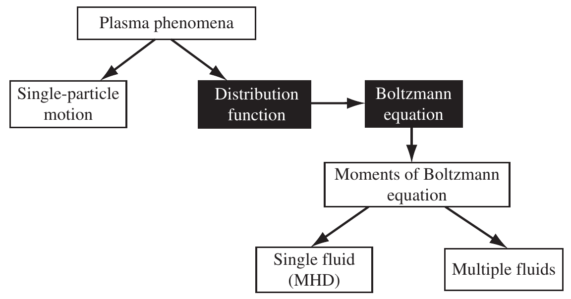
2.1 Hierarchy of plasma physics models

Kinetic description: microscopic properties. Fundamental variable: velocity distribution function \(f\).
Fluid description: it uses a few macroscopic quantities, averages of the distribution function (mean velocity, pressure/temperature). Valid for or near thermodynamic equilibrium.

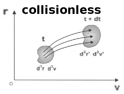
2.2 Vlasov equation

Liouville’s theorem: in absence of collisions, \(f\) is invariant along the trajectories in the 6D phase space.

\(\rightarrow\) Conservation of \(f(\vec{x},\vec{v},t)\) in phase space: \(Df/Dt=0\)
\(Df/Dt=0\) is called Vlasov equation considering:
- Convective derivative: \(D/Dt = \partial/\partial t + \vec{v}\cdot\partial/\partial\vec{x} + \vec{a}\cdot\partial/\partial\vec{v}\)
- Lorentz force: \(\vec{a}=\frac{q}{m}\left(\vec{E}+\vec{v}\times\vec{B}\right)\)
\[ \frac{Df}{Dt}=\left[\frac{\partial}{\partial t} + \vec{v}\cdot\frac{\partial}{\partial \vec{x}}+\frac{q_{\alpha}}{m_{\alpha}}\left(\vec{E}+\vec{v}\times\vec{B}\right)\cdot\frac{\partial}{\partial \vec{v}}\right]f_{\alpha}=0 \]

Conservation of the distribution function \(f\) (Bittencourt (2004)).

2.3 Fully-kinetic/Vlasov description

Fully-kinetic equations (electromagnetic case)

\[ \nabla\cdot\vec{E}=\frac{\rho}{\epsilon_0}\\ \nabla\cdot\vec{B}=0\\ \nabla\times\vec{E}=-\frac{\partial \vec{B}}{\partial t}\\ \nabla\times\vec{B}=\mu_0\vec{J}+\mu_0\epsilon_0\frac{\partial \vec{E}}{\partial t} \]

\[ \left[\frac{\partial}{\partial t} + \vec{v}\cdot\frac{\partial}{\partial \vec{x}}+\frac{q_{\alpha}}{m_{\alpha}}\left(\vec{E}+\vec{v}\times\vec{B}\right)\cdot\frac{\partial}{\partial \vec{v}}\right]f_{\alpha}=0\\ \rho=\sum\limits_{\alpha} q_{\alpha}\int\limits dv^3\,f_{\alpha}\\ \vec{J}=\sum\limits_{\alpha} q_{\alpha}\int dv^3\,\vec{v}f_{\alpha} \]

2.4 Electrostatic plasma approximation

Electrostatic (ES) plasma model

\[ \nabla^2\phi=-\frac{\rho}{\epsilon_0}\\ \left[\frac{\partial}{\partial t} + \vec{v}\cdot\frac{\partial}{\partial \vec{x}}+\frac{q_{\alpha}}{m_{\alpha}}\left(\vec{E}\right)\cdot\frac{\partial}{\partial \vec{v}}\right]f_{\alpha}=0\\ \rho=\sum\limits_{\alpha} q_{\alpha}\int\limits dv^3\,f_{\alpha} \]

2.5 Distribution functions in PIC

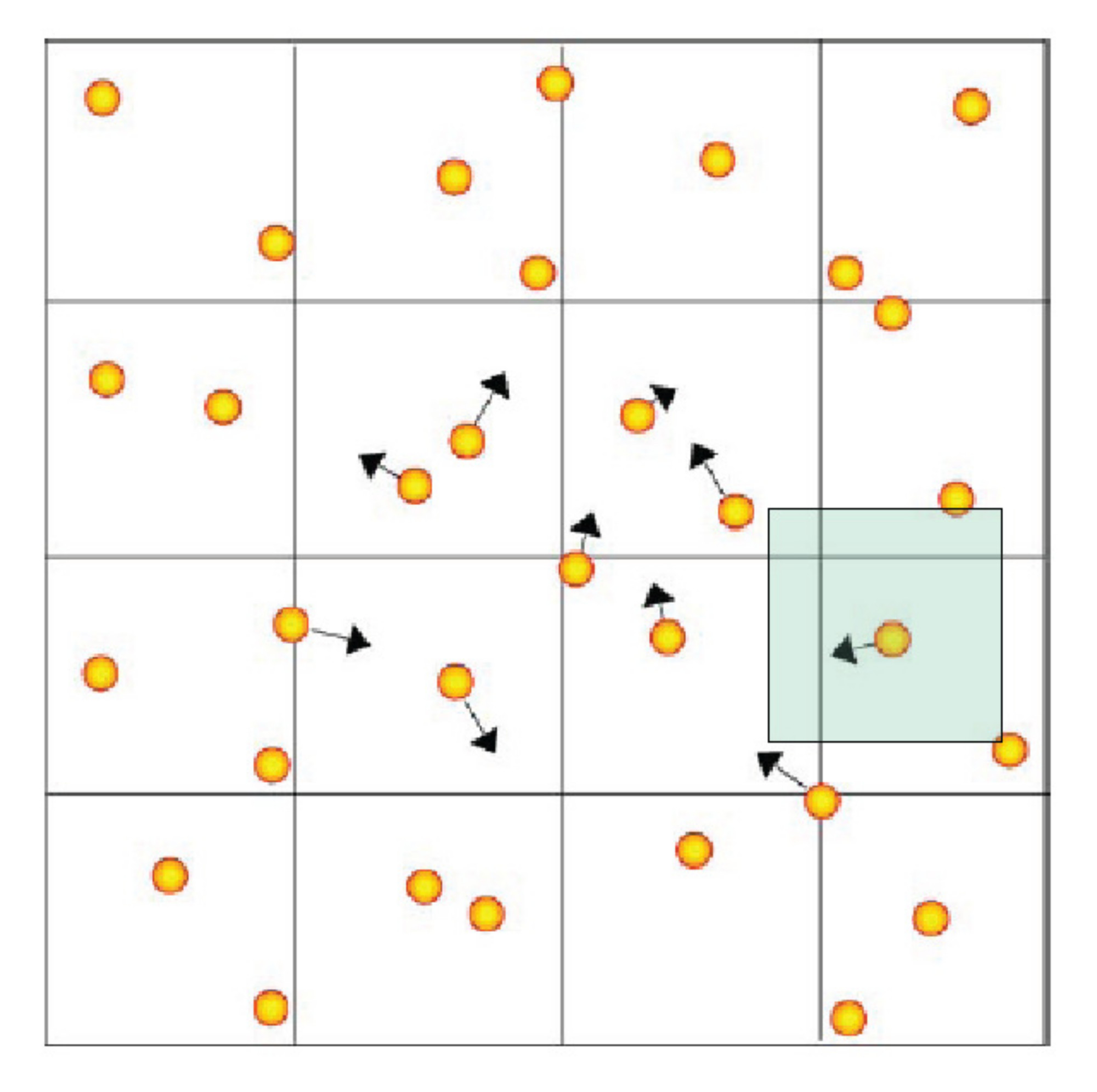
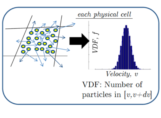
2.6 Vlasov vs PIC

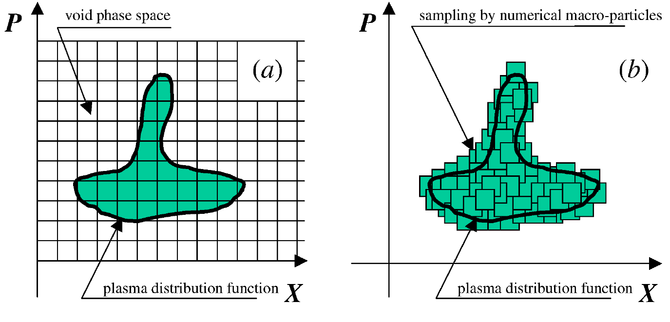
Phase space representation with PIC and Vlasov methods (Pukhov (2016)).

2.7 PIC vs Vlasov

Vlasov method is noise-free (PIC is noisy).
PIC can suffer from instabilities/numerical artifacts due to the finite number of particles.
Vlasov can suffer from instabilities due to the insufficient resolution of velocity space.
Vlasov method is computationally much more expensive than PIC methods (in particular regarding memory).

2.8 History

First methods to solve Vlasov eq. were developed in the 70’s
They were based on either Fourier/Hermite (spectral) transforms (very rare) or “splitting” schemes (very common). Lately also “unsplit” schemes.
Because of the required memory to solve the Vlasov eq, only 1D problems were treated until the 90s. First 2D applications toward the end of the 90s.
Only recently (this decade) full 3D Vlasov simulations have become feasible.

3 Electrostatic methods

3.1 Splitting algorithms

3.2 Hamiltonian flow and canonical variables

Let us denote a phase space point \(\vec{z}=(\vec{x},\vec{v})\). The Hamiltonian flow \(T^t\) (evolution operator) and its inverse are: \[ z(z_0,t)=T^tz_0, \\ z_0=T^{-t}z \]
This preserves the volume element in phase space \(dz=dz_0\).
The formal solution of the Vlasov equation can be written in terms of \(T^t\): \[ f(z,t)=T^tf_0(z)=f_0(T^{-t}z) \]

3.3 Hamiltonian for the electrostatic Vlasov eq.

The 1D electrostatic (Vlasov-Poisson) eq. has the Hamiltonian: \[ H=\frac{v^2}{2} + \Phi(x) \] (\(E=-\partial \Phi/\partial x\)). Thus the Vlasov eq. can be written as: \[ \frac{\partial f}{\partial t}=-[H,f]=\Lambda f \] where the Poisson bracket is defined as: \[ [H,f] = \frac{\partial H}{\partial x}\frac{\partial f}{\partial v} - \frac{\partial H}{\partial v}\frac{\partial f}{\partial x} \]
This way, the evolution of \(f\) can be described in terms of an evolution operator: \[ f(x,v,t)=T^tf_0(x,v),\;\;\; T^t=e^{\Lambda t} \]

3.4 Evolution operator for the Vlasov eq.

The 1D electrostatic Hamiltonian can be split as \[ H =H_1 + H_2, \\ H_1 = v^2/2, \\ H_2 =-\Phi(x) \] where the associated operators are explicit translations in \(x\) or \(v\) (Mangeney et al. (2002)): \[ e^{\Lambda_1 \tau}f(x,v) = f(x-v\tau,v) \\ e^{\Lambda_2 \tau}f(x,v) = f(x,v-E(x)\tau) \qquad(1)\]
Explicit form of Equation 1 and \(v=const.\) \[ T^tf(x)=e^{\Lambda_1 t}f(x)=f(x-vt),\;\;\Lambda_1=-v\frac{\partial}{\partial x}. \]

3.5 Evolution operator for the Vlasov eq.

In general (for \(\tau t =t/N\)): \[ e^{\Lambda \tau} = e^{\frac{\Lambda_2 \tau}{2}} e^{\Lambda_1 \tau} e^{\frac{\Lambda_2 \tau}{2}}+ \mathcal{O}(\tau^3) \] Baker-Campbell-Hausdorff (BCH) formula!
If the two operators \(\Lambda_1\) and \(\Lambda_2\) commute \[ e^{\Lambda \tau} = e^{(\Lambda_1 + \Lambda_2 )\tau} \]
Those kind of schemes preserving the phase space volume (and so conserving the energy and other invariants) are called symplectic integrators. For more details see Yoshida (1993), Donnelly and Rogers (2005).

3.6 Splitting scheme

The 1D electrostatic (Vlasov-Poisson) eq. can be split into: \[ \frac{\partial f_s}{\partial t} + v_x \frac{\partial f_s}{\partial x} = 0 \\ \frac{\partial f_s}{\partial t} + \frac{q_s}{m_s} E_x\frac{\partial f_s}{\partial v_x} = 0 \qquad(2)\]
This a system of 1st order (hyperbolic) advection eqs with the formal solution given as two shifts of \(f_s\), one in space and another in velocity: \[ f_s^a(x,v_x,t + \tau) = f_s(x - c_1\cdot v_x\cdot\tau , v,t) \\ f_s(x,v_x,t + \tau) = f_s^a(x, v - c_2\cdot(-E)\cdot\tau , t) \]
\(c_1\) and \(c_2\) are constants that are chosen depending on the specific algorithm.

3.7 Interpolation

3.8 Shift and interpolation

A solution of the 1D hyperbolic advection eq: \[ \frac{\partial f}{\partial t} + c\frac{\partial f}{\partial x} = 0 \] is (for \(c>0\)): \[ f(x,t) = f_0(x-ct) \] which is a simple shift (advection), \(f\) is advected without change of form from its arbitrary initial shape \(f_0=f(x,t=0)\).
Note that \(f_0(x-ct)\) is not necessarily known at grid points \(\Rightarrow\) is required.
The most popular interpolation is cubic splines (Mangeney et al. (2002)), a cubic polynomial where:
- Values at the interpolant \(=\) values of \(f\) at grid points
- 1st and 2nd derivatives of adjacent local interpolants are continuous at grid points.

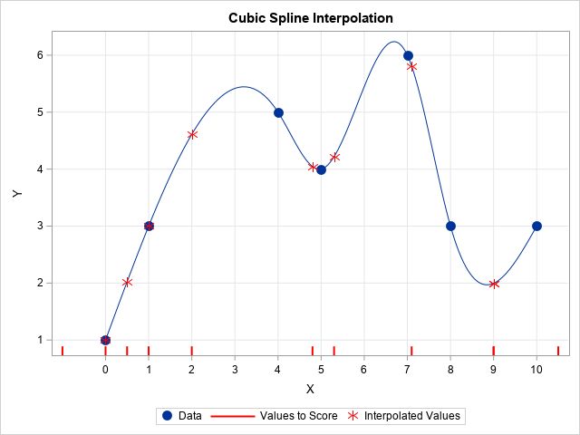
3.9 Splitting scheme: Shift and interpolation

3.10 Cubic splines

Given a function defined at grid points \(y_i=y(x_i)\), \(i=0,...N-1\), let focus on an interval \([x_j,x_{j+1}]\). The cubic interpolant is: \[ y = A y_j + B y_{j+1} + C y_j'' + D y_{j+1}'' \] with \[ A = \frac{x_{j+1} - x}{x_{j+1} - x_j},\;\; B=1-A\\ C = \frac{1}{6}(A^3 - A)(x_{j+1} - x_j)^2,\;\; D = \frac{1}{6}(B^3 - B)(x_{j+1} - x_j)^2, \] note \(A(x_j)=1\), \(A(x_{j+1})=0\) (B in the other way around).
By imposing continuity of the first and second derivatives at the boundaries of the intervals, we get an eq. for the unknown second derivatives \(y''\): \[ \frac{y_{j+1} - y_j}{x_{j+1} - x_j} - \frac{y_{j} - y_{j-1}}{x_{j} - x_{j-1}} = \frac{x_j - x_{j-1}}{6}y_{j-1}'' + \frac{x_{j+1} - x_{j-1}}{3}y_{j}'' + \frac{x_{j+1} - x_{j}}{6}y_{j+1}'' \]

3.11 Cubic splines

By imposing continuity of the first and second derivatives at the boundaries of the intervals, one gets a system of \(N-2\) linear equations in the \(N\) unknowns. There are several alternatives for choosing the last two constraints (Press et al. (2007)) (section 3.3)
The set of equations results in a tridiagonal system, each \(y_{j}''\) is coupled to only its nearest neighbors at \(j\pm1\).

3.12 Different methods

3.13 2nd order Cheng-Knorr

Cheng and Knorr (1976) proposed one of the classical methods to solve the electrostatic Vlasov-Poisson system:
- Solve \(\partial_t f + v\partial_x f=0\) for \(\tau/2\)
- Solve Poisson eq. for \(E\)
- Solve \(\partial_t f - E\partial_v f=0\) for \(\tau\)
- Solve \(\partial_t f + v\partial_x f=0\) for \(\tau/2\)
The corresponding shifts are: \[ f^a(x,v,t + \tau)= f(x - c_1\cdot v\cdot\tau , v,t) \\ f^b(x,v,t + \tau)= f^a(x, v - d_1\cdot (-E)\cdot\tau , t) \\ f(x,v,t + \tau)= f^b(x - c_2\cdot v\cdot\tau , v,t) \] with \(c_1=c_2=1/2\), \(d_1=1\) (Pohn, Shoucri, and Kamelander (2005)).

3.14 4th order symplectic

A symplectic (appliable when the Hamiltonian is separable) method and 4th order in time is (Pohn, Shoucri, and Kamelander (2005)). \[ f^a(x,v,t + \tau)= f(x - c_1\cdot v\cdot\tau , v,t) \\ f^b(x,v,t + \tau)= f^a(x, v - d_1\cdot (-E)\cdot\tau , t) \\ f^c(x,v,t + \tau)= f^b(x - c_2\cdot v\cdot\tau , v,t) \\ f^d(x,v,t + \tau)= f^c(x, v - d_2\cdot (-E)\cdot\tau , t) \\ f^e(x,v,t + \tau)= f^d(x - c_3\cdot v\cdot\tau , v,t) \\ f^f(x,v,t + \tau)= f^e(x, v - d_3\cdot (-E)\cdot\tau , t) \\ f(x,v,t + \tau)= f^f(x - c_4\cdot v\cdot\tau , v,t) \] with \[ c_1=c_4=\frac{1}{2(2-2^{1/3})},\;\;\; c_2=c_3 = \frac{1-2^{1/3}}{2(2-2^{1/3})}\\ d_1=d_3=\frac{1}{2-2^{1/3}},\;\;\; d_2 = -\frac{2^{1/3}}{2-2^{1/3}} \]

4 Applications

4.1 Applications

4.2 Bump-on-Tail instability

Initial function: \[ f_e=(1+\alpha\cos(kx))\left[(n_p/\sqrt{2\pi})\exp(-v^2/2)\right.\\ + \left.(n_b/\sqrt{2\pi})\exp(-(v-v_b)^2/(2v_t^2)\right]\nonumber \]

(Arber and Vann (2002)).

4.3 Two-stream instability

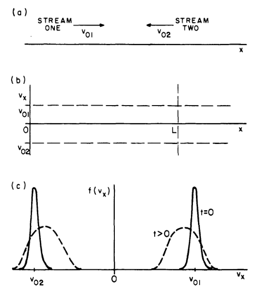
Setup of the two-stream instability (Birdsall and Langdon (1991)).

4.4 Two-stream instability

Domain: \(0\leq x<4\) and \(-5\leq v\leq 5\)
Initial distribution with two maxima at \(v=\pm\sqrt{2}\) and a periodic spatial perturbation: \[ f(x,v,t=0)=(1+\epsilon\cos(kx))v^2\frac{\exp(-v^2/2)}{\sqrt{2\pi}} \]
BGK modes (Bernstein, Greene, and Kruskal (1957)).

4.5 Two-stream instability

Phase space representation with PIC and Vlasov methods.

4.6 Earth’s magnetosphere

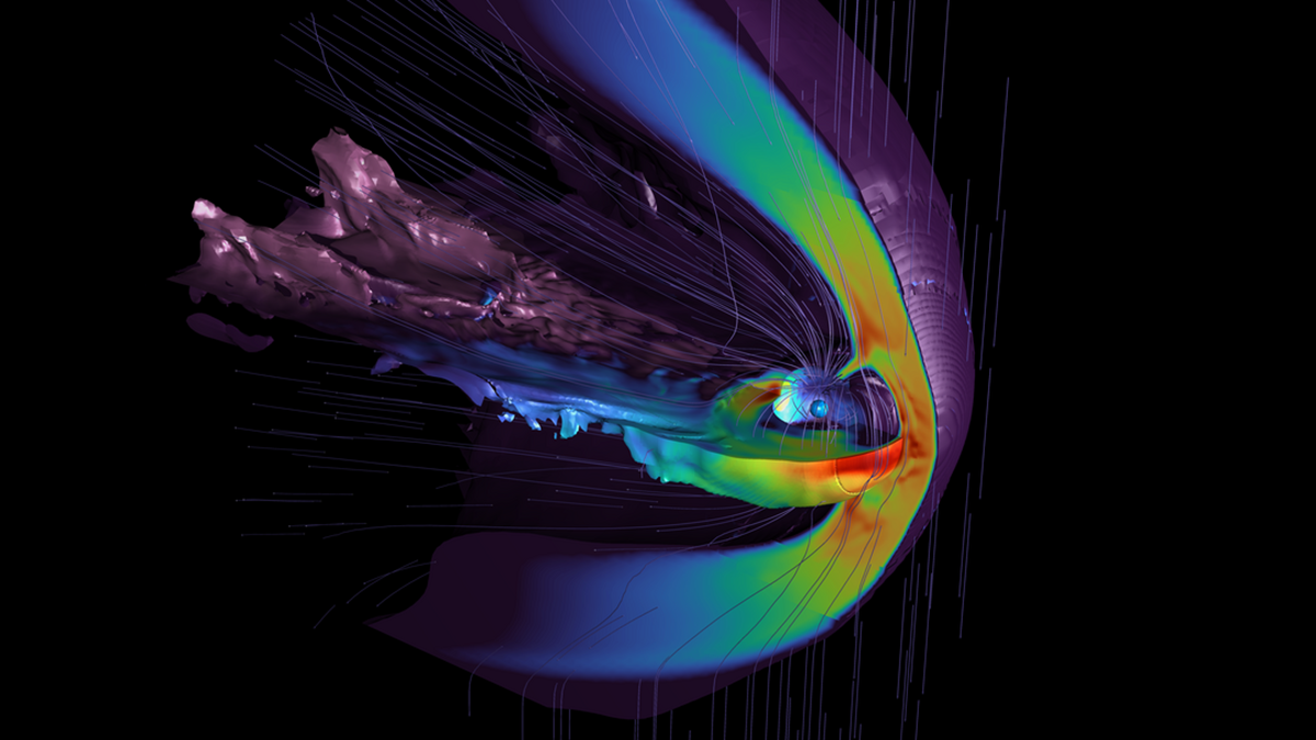
Vlasov methods in space physics and astrophysics, Palmroth et al. (2018)

4.7 Earth’s magnetosphere

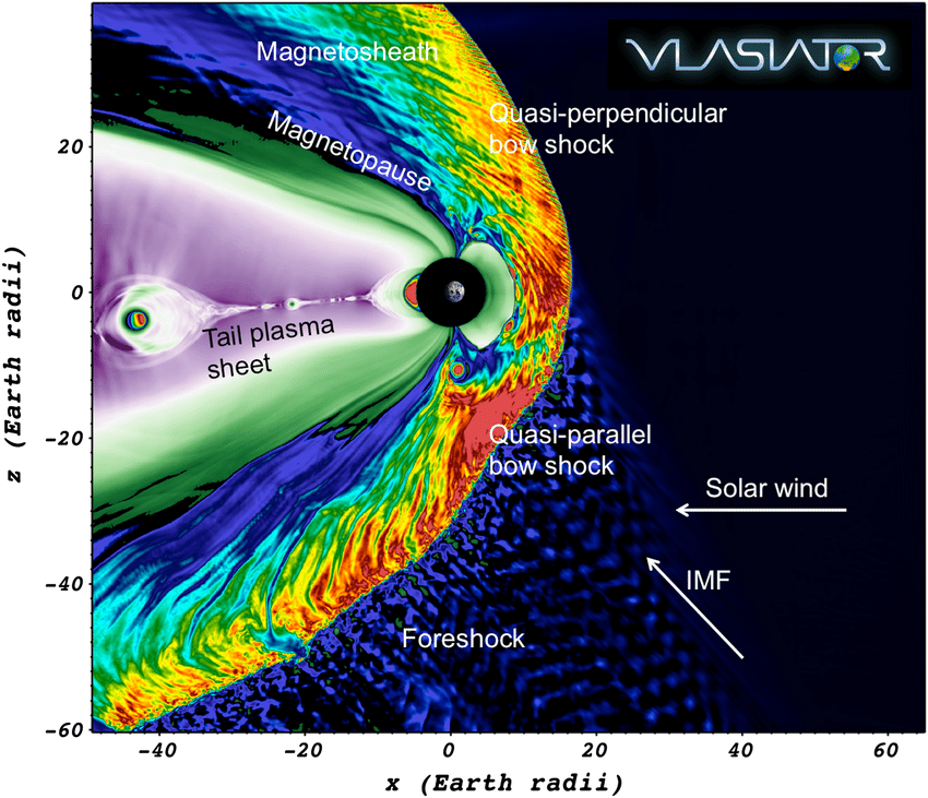
Ganse et al. (2023)

5 Numerical issues

5.1 Positivity

An ideal advection solver should have the following properties:
- The method should not introduce false extrema (preserve monotonicity)
- The methods should not accentuate existing extrema
Both properties imply that the method is positivity preserving (>\(f\)) and total variation diminishing (TVD) (Arber and Vann (2002)).
But a result of a theorem (Godunov’s) says that any higher-order (>1) scheme breaks those properties…
Many methods have been proposed to alleviate this problem, Van-Leer-Limited (VL, 2nd order, preserves positivity), Positive and Flux Conservative Method (PFC, (Filbet, Sonnendrücker, and Bertrand (2001))).
Piecewise Parabolic Method (PPM, 3rd order, preserves positivity), Flux-Corrected Transport (FCT, 4th order, preservers positivity by limiting flux).

5.2 Recurrence

For the free-streaming version (no field) of the electrostatic 1D Vlasov Poisson eq: \[ \frac{\partial f}{\partial t} + v\frac{\partial f}{\partial x}=0 \] the general solution is \(f(x,v,t) = f_0(x-vt, v)\) where \(f_0=f(x, v,t=0)\).
Initial condition: \[ f(x,v,0) = \frac{\exp(-v^2/2)}{\sqrt{2\pi}}(1+\epsilon\cos(kx)),\;\ \]
Analytical solution for the charge density (Pohn, Shoucri, and Kamelander (2005)): \[ \rho(x,v,0) = 1-\int_{-\infty}^{\infty}f(x-vt, v, 0) dv = \exp(-k^2t^2/2)\epsilon \cos(kx)\;\ \]

5.3 Recurrence

The numerical solution for the density, with \(N_v\) grid points and grid cell size \(\Delta v\) in velocity space, is: \[ n_e(x_i,t) = \sum_{j=0}^{N_v}f(x_i-v_j t, v_j, 0) = \sum_{j=0}^{N_v} f(x_i,v_j,0)\epsilon\cos(k(x_i-jt\Delta v)) \]

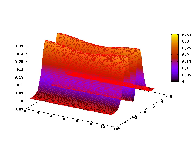
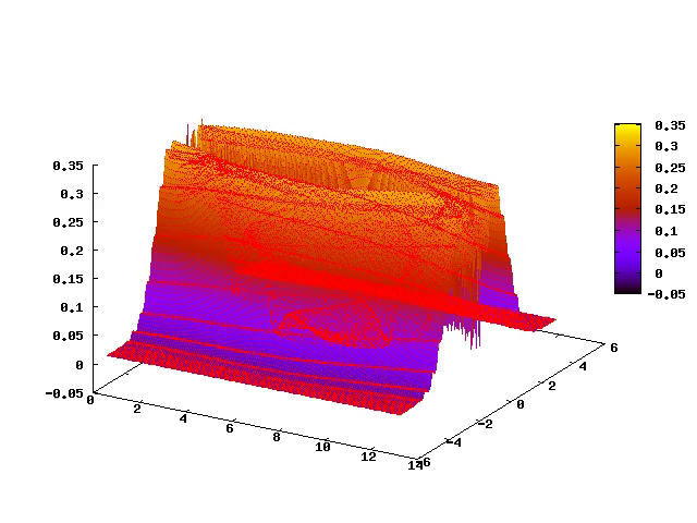
5.4 Recurrence

Due to the factor \(\cos(k(x_i-jt\Delta v))\), the numerical density \(n_e(x_i,t)\) is periodic in time, with recurrence time: \[ T_R=\frac{2\pi}{k \Delta v} \]

5.5 Recurrence in linear Landau damping

Initial function: \[ f_e= \frac{(1+\alpha\cos(kx))}{\sqrt{2\pi}}\exp(-\frac{v_e^2}{2}) \]

(Cheng and Knorr (1976)).

5.6 Filamentation

For the free-streaming version (no field) of the electrostatic 1D Vlasov Poisson: \[ \frac{\partial f}{\partial t} + v\frac{\partial f}{\partial x}=0 \] the solution is \(f(x,v,t) = f_0(x-vt, v)\) where \(f_0=f(x, v,t=0)\).
The velocity-derivatives of \(f\) will then be \[ \frac{\partial f}{\partial v} = \left.\frac{\partial f_0(\xi,v)}{\partial v}\right|_{\xi=x-vt} - t\frac{\partial f_0(x-vt,v)}{\partial x} \] indicating that the free streaming shears the initial phase space VDF as the time increases, the initial spatial structure is stretched into fine scale structures in velocity space without bound.

5.7 Filamentation

Some solution methods: A weak Fokker-Planck collision term to the RHS of the Vlasov eq. can relax fine velocity space structures
Filter method: after integrating \(f\) some number of timesteps, the following smoothing can be applied (Cheng and Knorr (1976)) \[ \bar{f}(x_j,v) = \int_{-\infty}^{\infty} f(x_j, v-v') \exp(-(v'/v_c)^{2n}) dv' \] in practice this smoothing is performed in the Fourier space (Klimas (1987)).

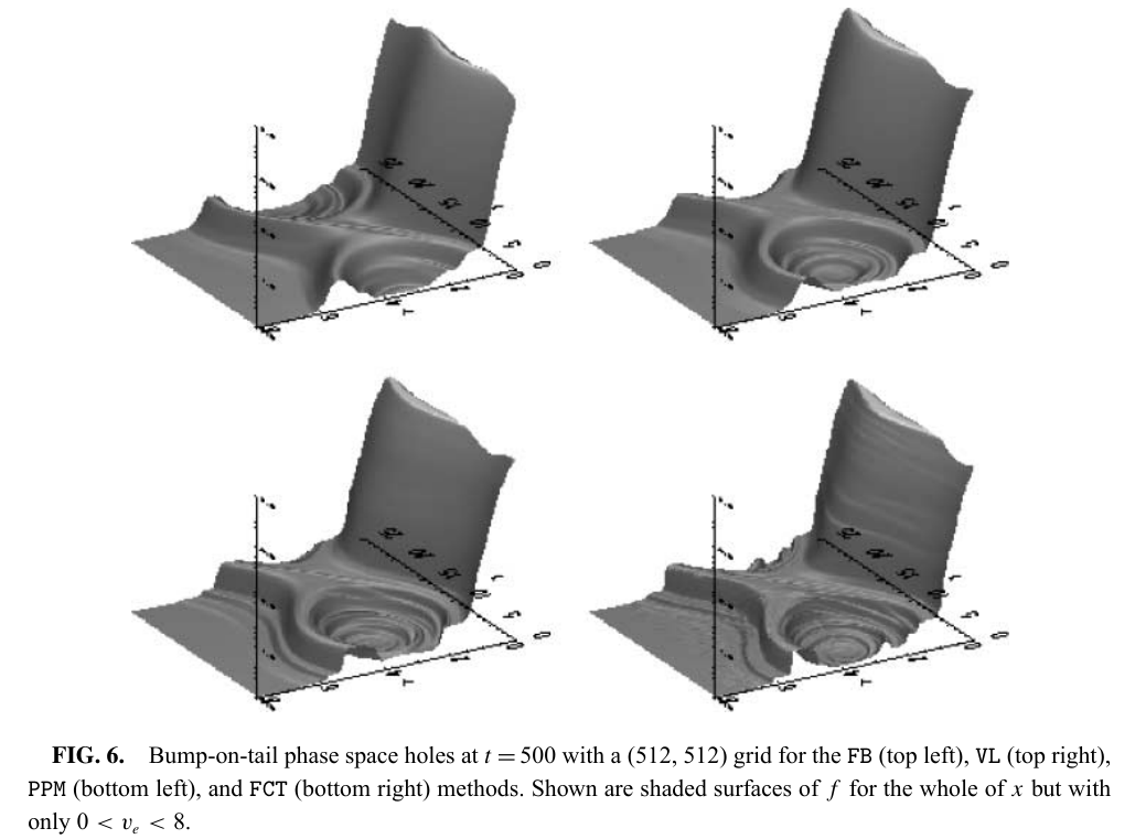
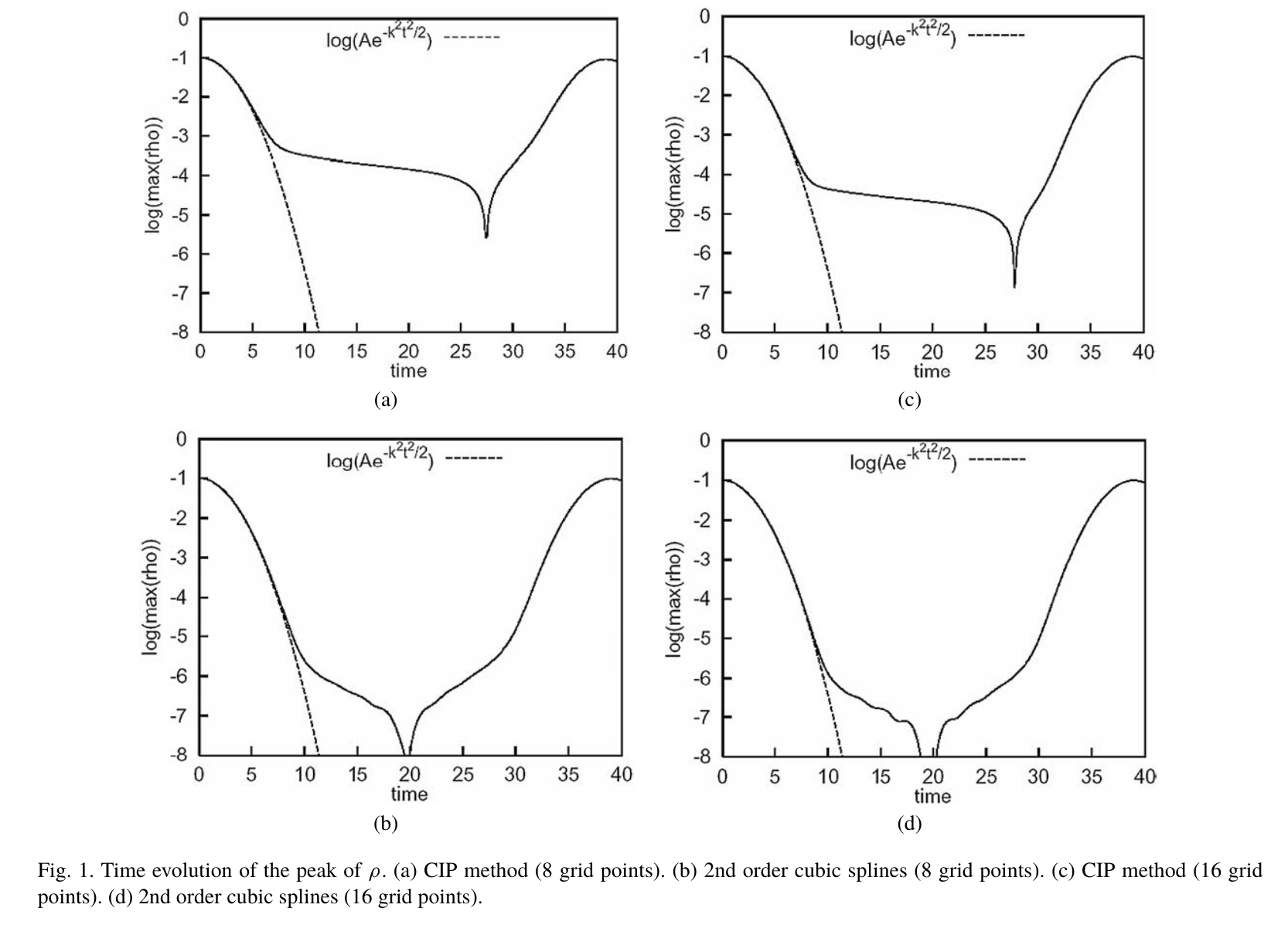
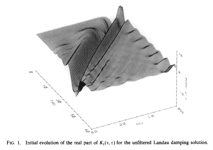
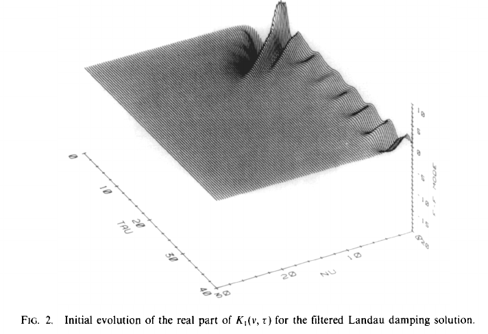
5.8 Filamentation for the non-Linear Landau damping

(Cheng and Knorr (1976))

5.9 Filamentation

Filtering \(f\) with a Gaussian distribution. Comparison for a Landau damping problem (Klimas (1987)).

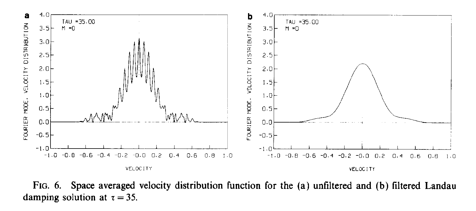
(Klimas (1987)).

5.10 Filamentation

6 Introduction to dispersion solvers

6.1 Introduction

6.2 What is the dispersion?

Any relation between wave frequency \(\omega\) and its wavelength \(\lambda\)
Typically used wavenumber \(k = \frac{2\pi}{\lambda}\)
For medium, the relation is an implicit function \(\Phi = \Phi(\omega,k)\)

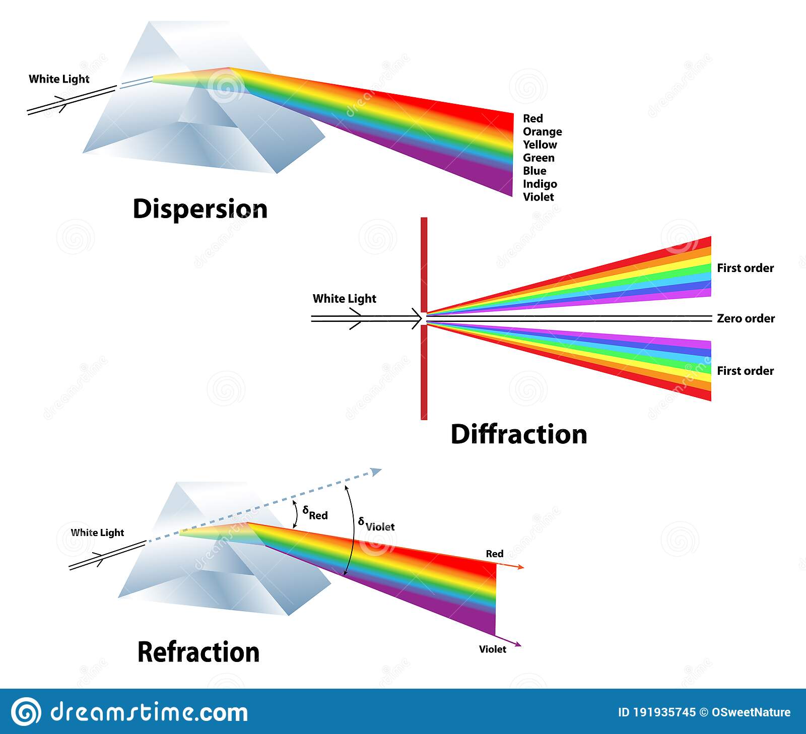
Comparison of dispersion, diffraction, and refraction in solids.

6.3 Why use a linear approach?

Fluid turbulence cascade (Narita (2012))

Wave-wave interaction . Waves satisfy \(\vec{k}_1+\vec{k}_2 = \vec{k}_3\) and \(\omega_1 + \omega_2 = \omega_3\). Left panel is characteristic of solar wind turbulence. Right panel is characteristic of foreshock turbulence.

6.4 Plasma properties of our interest

Oscillating wave \[ E(\omega, k) = E_0 e^{-i(kx - \omega t)} \] with assumption that \(k\) is real and \[ \omega = \omega_r + i \omega_i = \omega_r + i \gamma \] \[ E(\omega, k) = E_0 e^{-i(kx - (\omega_r + i\gamma) t)} = E_0 e^{\gamma t} e^{-i(kx - \omega_r t)}. \]
Relation \(\omega = k c (\nu = c / \lambda)\) is valid only for electromagnetic waves in vacuum.
Any plasma described by dispersion tensor (electric permittivity) \[ \nabla \cdot (\hat{\epsilon} \vec{E}) = \rho. \]
Solutions of \(\mathrm{det}(\hat \epsilon(\omega, k)) = 0\) are waves (set of (\(\omega, k\))) that might be present in the plasma.
How the tensor looks like?

6.5 Plasma properties of our interest

Solutions of dispersion relation \((\omega, k)\) are not a finite set of numbers
They form “dispersion branches” - continuous set (curves) of solutions in \(\omega - k\)
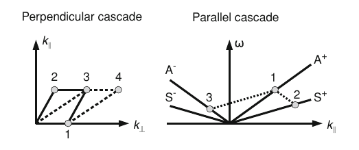
Example of Bernstein waves

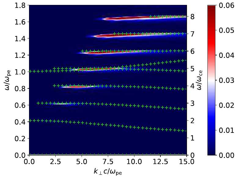
Green pluses: real solutions, color scale: wave growth rates. (Benáček & Karlický 2019).

7 Linearization

7.1 General approach

Linear analysis (linearization) is a general method applicable to any system of PDEs.
In plasma physics, we apply this method to the Maxwell-Lorentz system of eqs. (where the Lorentz force can be represented via the Vlasov, two-fluid or MHD models) in order to find linear (small-amplitude) plasma waves.

7.2 General approach

Let the dependent variables: \[ \{f(\vec{x},t), g(\vec{x},t), h(\vec{x},t),...\} \]
If any perturbation is applied to one of those variables, then solving the system of PDEs will provide the response of all the other dependent variables.
For example, let us assume a perturbation: \[ f=f_0 + \epsilon f_1 + O(\epsilon^2 f_2) \] where \(\epsilon\ll1\) and \(\epsilon|f_1|\ll |f_0|\).
This implies, for example, \[ g=g(f)=g(f_0 + \epsilon f_1)\\ g=g_0 + \epsilon g_1 +\epsilon^2 g_2+... \] so that the variables can be written as (considering \(\epsilon\)’s as implicit): \[ f= f_0 + f_1\\ g= g_0 + g_1 + O(g_2) \\ h= h_0 + h_1 + O(h_2) \]

7.3 General approach

Continuity equation \[ \frac{\partial n}{\partial t} + \nabla \cdot (n \vec{v}) = 0. \]
Each PDE is rewritten with all dependent quantities expanded to first order. Example for the continuity eq: \[ \frac{\partial(n_0 + n_1)}{\partial t} + \nabla\cdot \left[(n_0 + n_1)(\vec{V}_0 + \vec{V}_1) \right]=0 \qquad(3)\]
The equilibrium solution is substracted from the expanded Equation 3 so that: \[ \frac{\partial(n_1)}{\partial t} + \nabla\cdot \left(n_1\vec{V}_0 + n_0\vec{V}_1 + n_1\vec{V}_1 \right)=0, \qquad n_1\vec{V}_1 \rightarrow 0 \qquad(4)\] where the last term is discarded because it is the product of two first order quantities, and so of order \(\epsilon^2\).
Note that all the other terms are of order \(\epsilon\).
Equation 4 is the linearized (continuity) eq. (like the differential of the original eq.).

8 Electrostatic dispersion relation

8.1 Electrostatic approaches

8.2 Electrostatic Vlasov eq.

Vlasov-Poisson (electrostatic) plasma model.
The equilibrium solution for \(f\) of the Vlasov-Poisson eq. is the Maxwellian distribution (for each species): \[ f_0(\vec{v}) = \frac{n_0}{(2\pi v_{th}^2)^{3/2}}\exp\left(-\frac{v^2}{2v_{th}^2}\right); \quad f_1(\vec{v}) \equiv \mathrm{perturbation} \qquad(5)\] with \(v_{th}=\sqrt{k_BT/m}\). \(\vec{E}_0=0\)
The linearized Vlasov eq. is: \[ \frac{\partial f_1(\vec{x},\vec{v},t)}{\partial t} +\vec{v}\cdot\frac{\partial f_1(\vec{x},\vec{v},t)}{\partial \vec{x}} +\frac{e}{m}\vec{E}_1(\vec{x},t)\cdot \frac{\partial f_0(\vec{v})}{\partial \vec{v}} =0 \] \[ \nabla\cdot\vec{E}_1(\vec{x},t)=\rho_1(\vec{x},t)/\epsilon_0,\;\;\;\vec{E}_1=-\nabla\phi_1 \]
The rigorous solution of this equations needs to invoke a Laplace-Fourier transform (initial value problem) instead of a simpler Fourier transform (normal mode problem), but for the simplest asymptotic solution the latter is enough, i.e: \[ h_1(\vec{x},t) = h_1(\vec{k},\omega)\exp(i(\vec{k}\cdot\vec{x}-\omega t)),\;\;\;\text{with }\omega=\omega_r + i\gamma \]

8.3 Electrostatic Vlasov eq.

Then, the linearized electrostatic Vlasov eq. becomes: \[ -i(\omega - \vec{k}\cdot\vec{v})f_1(\vec{k},\vec{v},\omega) = \frac{e}{m}\phi_1(\vec{k},\omega) i\vec{k}\cdot \frac{\partial f_0(\vec{v})}{\partial \vec{v}} \]
The perturbed density, \(n_1(\vec{k},\omega)=\int f_1(\vec{k},\vec{v},\omega) d^3\vec{v}\), becomes, \[ n_1(\vec{k},\omega) = \frac{e}{m}\phi_1(\vec{k},\omega) \int \frac{d^3v}{\vec{k}\cdot\vec{v} - \omega}\vec{k}\frac{\partial f_0(\vec{v})}{\partial \vec{v}} \]
At this point it is customary to introduce the electric susceptibility \(\chi\) (related to the dielectric constant \(\epsilon_r\) via \(\chi = \epsilon_r -1\), so that \(\vec{D}=\epsilon_0(1+\chi_e)\vec{E}=\epsilon_r\epsilon_0\vec{E}=\epsilon\vec{E}\), so that we have (Gary (1993)): \[ n_1(\vec{k},\omega) = -\frac{\epsilon_0k^2 \phi_1(\vec{k},\omega)}{e} \chi(\vec{k},\omega) \\ \chi(\vec{k},\omega) = - \frac{\omega_p^2}{n_0k^2} \int \frac{d^3v}{\vec{k}\cdot\vec{v} - \omega}\vec{k}\frac{\partial f_0(\vec{v})}{\partial \vec{v}} \]

8.4 Electrostatic Vlasov eq.

We take Poisson equation \[ \nabla^2 \phi_1(\vec{x},t) = \frac{1}{\epsilon_0}\sum_s \rho_1^s(\vec{x},t), \]
Replacing \(n_1\) into the perturbed Poisson eq: \[ k^2\phi_1(\vec{k},\omega) = \frac{e}{\epsilon_0} \sum_s n_1^s(\vec{k},\omega) \] we get, after integrating by parts and defining \(v_k=\vec{v}\cdot\vec{k}/k\), \[ 1+\sum_s\chi_s(\vec{k},\omega)=0\\ 1 + \sum_s \frac{\omega_{ps}^2}{n_{0s} k^2} \int \frac{dv_k}{v_k - \omega/k}\frac{\partial f_0(v_k)}{\partial v_k} = 0 \qquad(6)\] which is a dispersion relation, linking \(\omega=\omega_r+i\gamma\) with \(\vec{k}\).

8.5 Plasma dispersion function

8.6 Electrostatic Vlasov eq.

For Maxwell velocity distribution \[ f_0(\vec{v}) = \frac{n_0}{(2\pi v_{th}^2)^{3/2}}\exp\left(-\frac{v^2}{2v_{th}^2}\right) \qquad(7)\] \[ \int \frac{dv_k}{v_k - \omega/k}\frac{\partial f_0(v_k)}{\partial v_k} \]
Plasma dispersion function \[ \frac{1}{\sqrt{\pi}}\int_{-\infty}^{\infty}\frac{\exp(-x^2)}{x-\zeta}dx = Z(\zeta) \]
For a Maxwellian distribution function (Equation 7), the electric susceptibility of the electrostatic dispersion relation in Equation 6 becomes: \[ \chi_s(\vec{k},\omega)=-\frac{1}{2(k\lambda_{Ds})^2}Z'(\zeta_s) \qquad(8)\] where \(\lambda_{Ds}=\sqrt{\epsilon_0k_BT_s/(n_{0s}e^2)}\) is the Debye length of the species \(s\), with argument: \[ \zeta_s = \frac{\omega}{\sqrt{2}kv_{th,s}} \]

8.7 The plasma dispersion function

Plasma dispersion (Z) function: \[ Z(\zeta)=\frac{1}{\sqrt{\pi}}\int_{-\infty}^{\infty}\frac{\exp(-x^2)}{x-\zeta} dx \]
It is related to the error function of complex argument: \[ {\rm erf}(\zeta) = \frac{2}{\sqrt{\pi}}\int_{0}^{\zeta}dx\exp(-x^2)\\ {\rm erfc}(\zeta) = 1- {\rm erf}(\zeta)\\ Z(\zeta) = i \sqrt{\pi}\exp(-\zeta^2){\rm erfc}(-i\zeta) \]
Properties: \[ Z'(\zeta) = -2( 1 + \zeta Z(\zeta)) \]

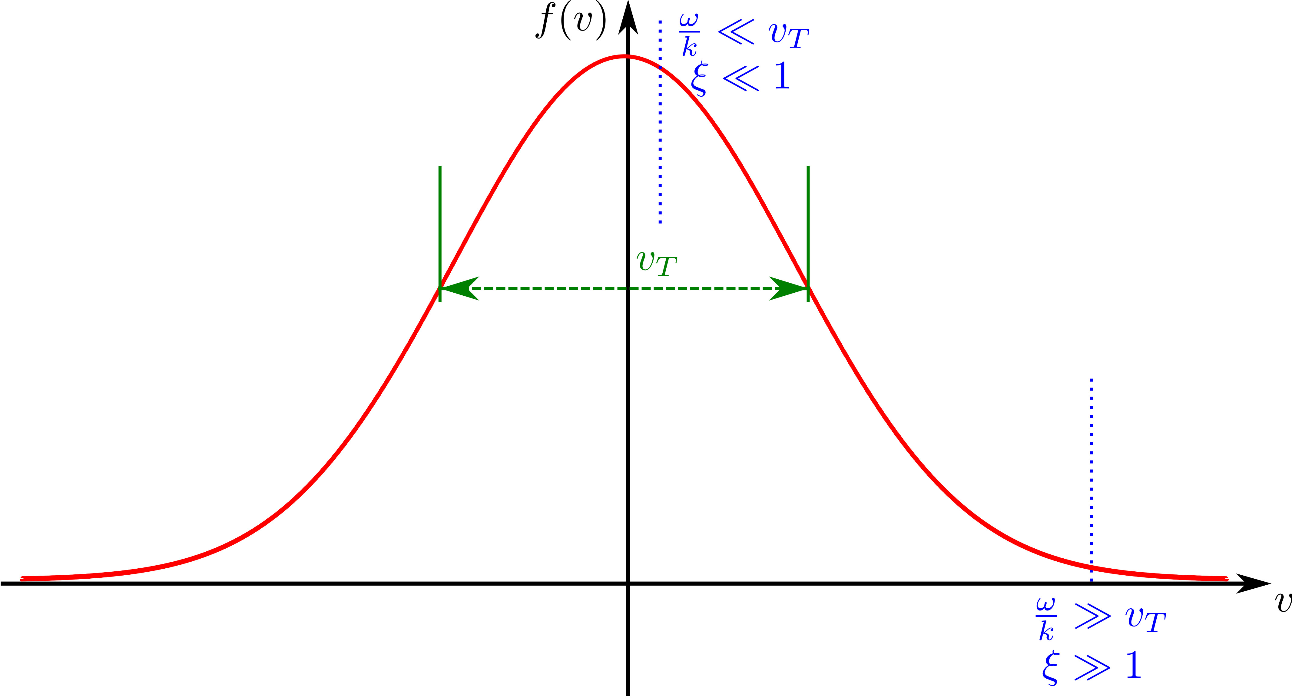
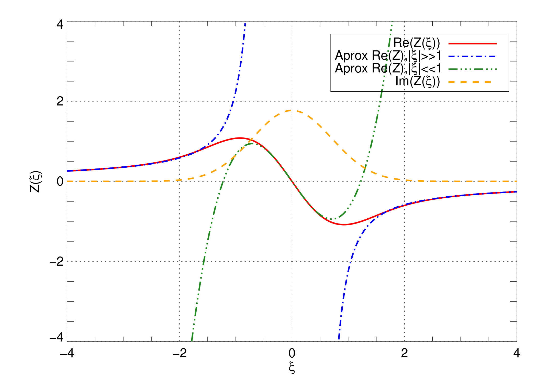
8.8 The plasma dispersion function

If \(\zeta<1\), \(exp(-x^2)\) is significant at the resonance \(\omega_r=\vec{k}\cdot\vec{v}\), particles satisfying this condition are said to be in Landau resonance with the wave, such that \(\vec{E}_1\cdot\vec{v}\) is constant.

8.9 Landau procedure

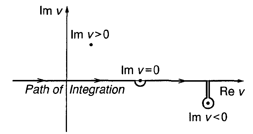
The integrand of \(Z\) has a singularity at \(\omega=\vec{k}\cdot\vec{v}\), so the contour of integration for \(v_k=\vec{v}\cdot\vec{k}/k\) must be specified.
Landau (1946) proposed the right solution: the contour must pass below the singularity, regardless the value of \(\gamma\).
For unstable modes, the singularity lies in the upper half \(v_k\) plane, a direct integration along the real \(v_k\) axis satisfies the Landau prescription.
For stable or damped waves with \(\gamma<0\), the Landau contour must involve an additional contribution around the singularity, the result is a function that is an analytical continuation of the function for the case \(\gamma>0\).

8.10 Landau procedure

The correct implementation of the Landau procedure involves a Laplace transform \[ \psi(p)= \int_0^{\infty}\psi(t)\exp(-pt)dt \]
If \(\gamma\ll \omega_r\) one may approximate the Landau contour by a straight line and a semicircular path around the pole (Plemelj formula) \[ \int\frac{dv_k}{v_k - \omega/k}g(v_k) = P\int\frac{dv_k}{v_k - \omega/k}g(v_k) + i\pi g(v_k)|_{v_k=\omega_r/k} \]

8.11 Solution method

The electrostatic dispersion relation (and also the general magnetized case) is a transcendental equation for the complex variable \(\omega\) in terms of the real wavevector \(\vec{k}\), which can be written as \(\hat{\epsilon}(\omega_r+i\gamma,\vec{k})=0\)
Solving the determinant of the dispersion \[ Det (\hat{\epsilon}(\omega_r+i\gamma,\vec{k})) = D(\omega_r+i\gamma,\vec{k}) \]
For each choice of plasma parameters, this equation has many solutions \(\omega=\omega(\vec{k})\).
The solution method is based first on splitting \(D\) thus: \[ D(\omega_r+i\gamma,\vec{k}) = \textrm{Re}[D(\omega_r+i\gamma,\vec{k})] + i\textrm{Im}[D(\omega_r+i\gamma,\vec{k})] \]
Then, the solutions of the dispersion relation will be located where the contours at level 0 of the real functions \(\textrm{Re}(D)\) and \(\textrm{Im}(D)\) satisfy simultaneously: \[ \textrm{Re}[D](\omega_r,\gamma,\vec{k}) = 0\\ \textrm{Im}[D](\omega_r,\gamma,\vec{k}) = 0 \] i.e., the solutions are at the intersections of contours levels at 0.

8.12 Solution method

The intersections \((\omega, \gamma)\) of the contour levels at 0 can be found via improved versions of the Newton-Raphson method for a given \(\vec{k}_0\), provided a good enough initial guess, leading to \(\omega(\vec{k}_0),\gamma(\vec{k}_0)\)
Then the process is repeated for a \(\vec{k}_0+\Delta\vec{k}\), using as a initial guess the same value found in the previous step, leading to a \(\omega(\vec{k}_0+\Delta\vec{k}),\gamma(\vec{k}_0+\Delta\vec{k})\), and so on.
Two set of curves \(\omega=\omega(k)\) and \(\gamma=\gamma(k)\) are obtained for each one of the initial intersections.

Green pluses: real solutions, color scale: wave growth rates. (Benáček & Karlický 2019).

9 Examples

9.1 Electron plasma waves

At frequencies \(\omega>\omega_{pe}\), ions can be considered immobile.
It is possible to use the asymptotic expansion of \(Z'(\zeta_e)\) for \(k\ll 1/(\lambda_{De})\) and \(\zeta_e\gg 1\) so we get the dispersion relation and damping rate of Langmuir or electron plasma waves (Gary (1993)): \[ \omega_r^2 = \omega_{pe}^2 + 3k^2 v_{th,e}^2\\ \gamma = -\left(\frac{\pi}{8}\right)^{1/2}\frac{1}{(k\lambda_{De})^3}\frac{\omega_r^2}{\omega_{pe}}\exp\left(-\frac{\omega_r^2}{2k^2v_{th,e}^2}\right) \]

9.2 Electron plasma waves

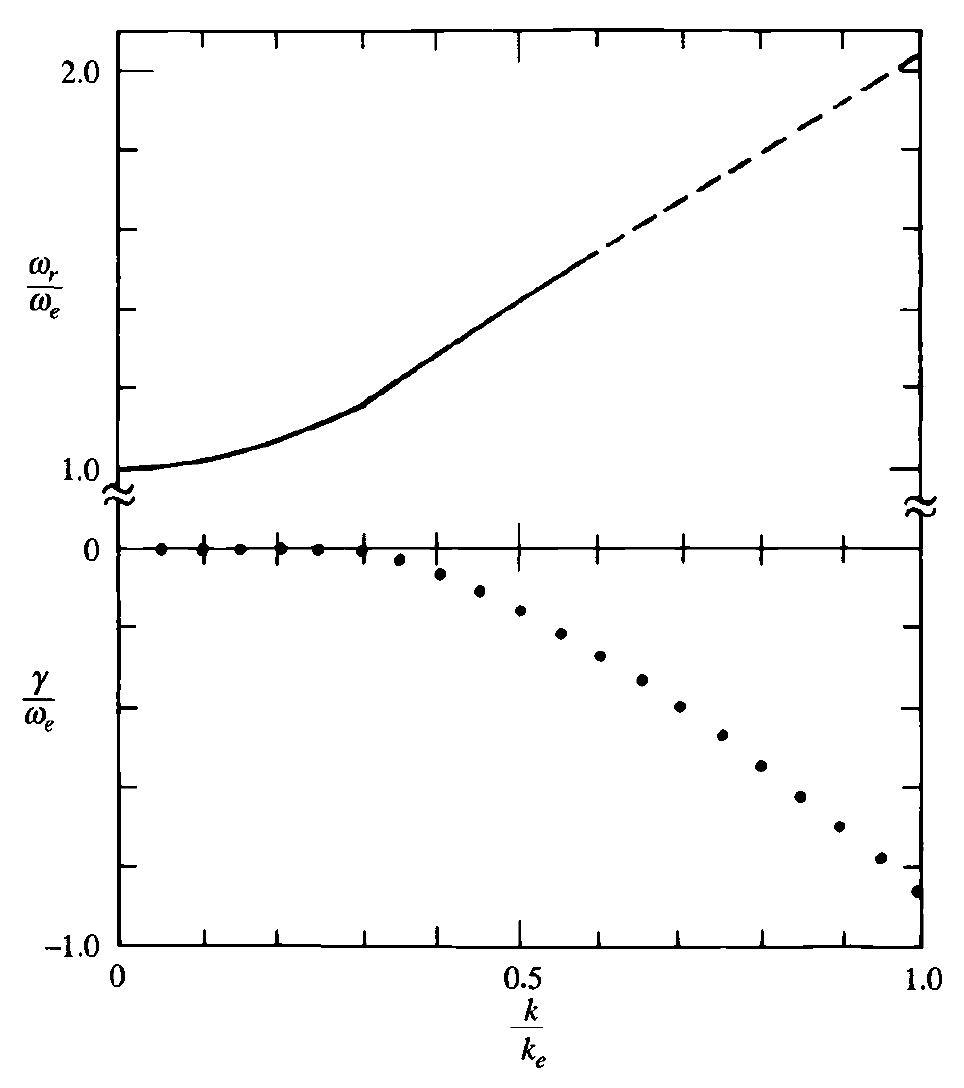
Electron plasma waves. Top panel: real frequency. Bottom panel: damping rate (Gary (1993)).

9.3 Ion acoustic waves

Ion acoustic-like (i.e.: \(\omega_r/k\sim\) constant) are heavily damped \(\gamma\sim \omega_r\).
For \(T_e\gg T_i\), \(\zeta_i>1\) and \(\zeta_e\ll 1\), we can use the corresponding asymptotic expansions of \(Z(\zeta)\) so that (Baumjohann and Treumann (1997)): \[ \omega_r^2=\frac{\omega_{pi}^2}{1+(k\lambda_{De})^2}\left[1 + \frac{3T_i}{T_e}(1+(k\lambda_{De})^2\right] \]
In the long wavelength limit \(k\lambda_{De}\ll1\), the phase speed is the \(c_s=\sqrt{(T_e+3T_i)/m_i}\) and \[ \omega_r=c_s k \]
The damping rate is: \[ \gamma=-\left(\frac{\pi}{8}\right)^{1/2} \left[\left(\frac{m_e}{m_i}\right)^{1/2} + \left(\frac{T_e}{T_i}\right)^{3/2} \exp\left(-\frac{T_e}{2T_i} - \frac{3}{2} \right)\right] \]

9.4 Ion acoustic waves

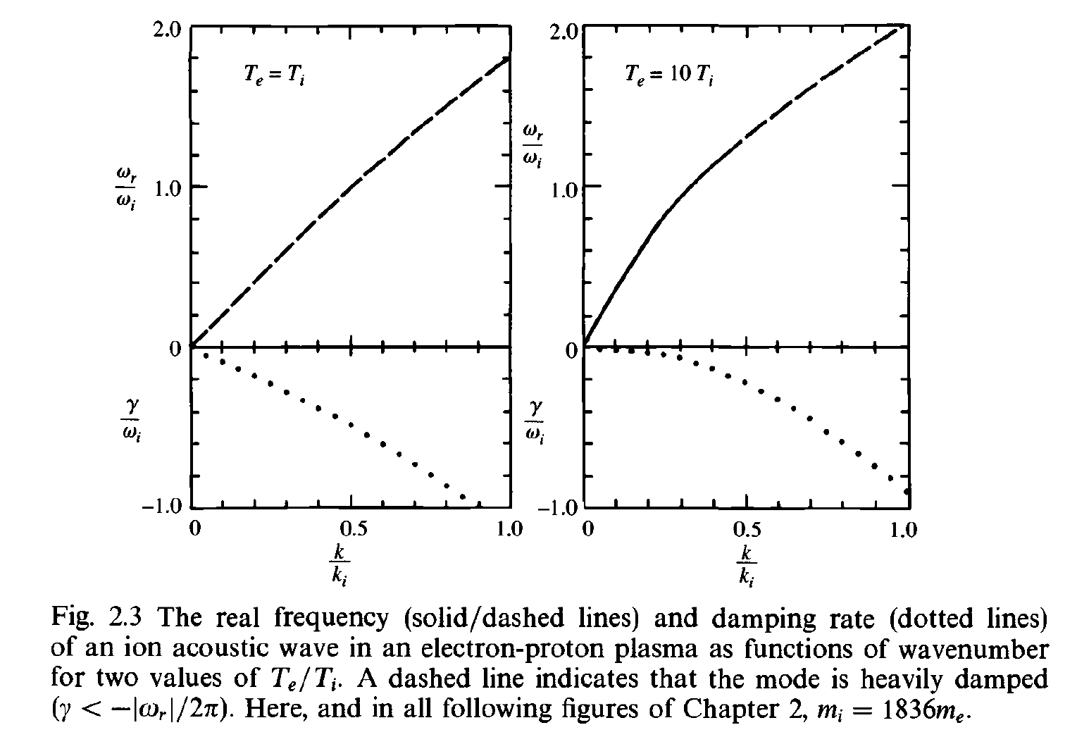
Ion acoustic waves (Gary (1993)).

10 General dispersion relation

10.1 General dispersion relation

10.2 General plasma dispersion relation

Taking the derivative of Ampére’s law, and eliminating \(\vec{B}\) via Faraday’s law, we get the general wave equation: \[ \nabla^2\vec{E} - \nabla(\nabla\cdot\vec{E}) - \mu_0\epsilon_0\frac{\partial^2\vec{E}}{\partial t^2}= \mu\frac{\partial \vec{J}}{\partial t} \]
We assume a linear relation between the current density and electric field (valid for small perturbations), corresponding to a time-varying : \[ \vec{J}=\int d^3x'\int_{-\infty}^t dt' \bar{\sigma}(\vec{x}, \vec{x}', t, t' )\cdot\vec{E} \]
The integration in time from \(-\infty\) to \(t\) contains the concept of causality (history of the plasma contributes to its response at time \(t\)), while the future behaviour is determined by the solution of Maxwell’s eqs.
The conductivity tensor \(\sigma\) describes all properties of the plasma, closing the Maxwell system of eqs. It depends, therefore, on the choice of plasma model.

10.3 General plasma dispersion relation

Linear general wave equation and Ohm’s law (which becomes dependent only on the relative position and time)

\[ \nabla^2\vec{E}_1 - \nabla(\nabla\cdot\vec{E}_1) - \mu_0\epsilon_0\frac{\partial^2\vec{E}_1}{\partial t^2}= \mu\frac{\partial \vec{J}_1}{\partial t}\\ \vec{J}_1=\int d^3x'\int_{-\infty}^t dt' \bar{\sigma}(\vec{x}-\vec{x}', t- t' )\cdot\vec{E}_1 \qquad(9)\]

Plane wave Ansatz: \[ \vec{E}_1(\omega,\vec{k}) = \vec{E}_1^0(\omega,\vec{k}) \exp(i\vec{k}\cdot\vec{x} - i\omega t) \] This reduces the system of Equation 9 to: \[ \left[\left(k^2 - \frac{\omega^2}{c^2}\right) \mathbb{1} - \vec{k}\vec{k} -i\omega \mu_0 \bar{\sigma}(\omega,\vec{k}) \right] \vec{E}_1^0(\omega,\vec{k})= 0 \qquad(10)\]

10.4 General plasma dispersion relation

The non-trivial solutions of Equation 10 are given by: \[ D(\omega, \vec{k})= {\rm Det}\left[\left(k^2 - \frac{\omega^2}{c^2}\right) \mathbb{1} - \vec{k}\vec{k} -i\omega \mu_0 \bar{\sigma}(\omega,\vec{k}) \right] = 0 \]
By introducing the dielectric tensor \(\epsilon\) which relates the electric induction (or electric displacement field) \(\vec{D}\) to \(\vec{E}\) such that \[ \vec{D}_1=\bar{\epsilon}\vec{E}_1 \] we can rewrite the electric conductivity \(\sigma\) in terms of \(\epsilon\) \[ \bar{\epsilon}(\omega,\vec{k})=\mathbb{1} + \frac{i}{\omega\epsilon_0}\bar{\sigma}(\omega,\vec{k}) \]
Thus, the dispersion relation can be written in this way: \[ D(\omega, \vec{k})= {\rm Det}\left[\frac{k^2c^2}{\omega^2}\left(\frac{\vec{k}\vec{k}}{k^2}-\mathbb{1}\right) +\bar{\epsilon}(\omega,\vec{k}) \right] = 0 \]
Note that this expression has been derived using uniquely the Maxwell equations \(\Rightarrow\) it is independent on the plasma model.

11 Magnetized dispersion relation

11.1 Electromagnetic Vlasov eq.

Linearized Vlasov equation for a magnetized plasma: \[ \left(\frac{\partial }{\partial t} + \vec{v}\cdot + \frac{e}{m}\vec{v}\times\vec{B}_0\cdot\frac{\partial}{\partial \vec{v}} \right)\cdot f_1(\vec{x},\vec{v},t) = -\frac{q}{m}\left(\vec{E}_1(\vec{x},t) + \vec{v}\times\vec{B}_1(\vec{x},t)\right) \frac{\partial f_0(\vec{x}) }{\partial \vec{v}(t)} \]
The LHS is a total derivative along a particle phase space orbit: \[ \frac{d f_1(\vec{x}(t),\vec{v}(t),t)}{dt} = -\frac{q}{m}\left(\vec{E}_1(\vec{x}(t),t) + \vec{v}(t)\times\vec{B}_1(\vec{x}(t),t)\right)\cdot \frac{\partial f_0(\vec{v}(t)) }{\partial \vec{v}(t)} \]
The formal solution of this equation is obtained by integrating over the entire history of phase space trajectories: \[ f_1(\vec{x}(t),\vec{v}(t),t) = -\frac{q}{m}\int_{-\infty}^tdt'\left(\vec{E}_1(\vec{x}(t'),t') + \vec{v}(t')\times\vec{B}_1(\vec{x}(t'),t')\right)\cdot \frac{\partial f_0(\vec{v}(t')) }{\partial \vec{v}(t')} \]

11.2 Characteristics of the Vlasov eq.

In the linear approximation we have now to determine the particle orbits (characteristics of the Vlasov eq) in the equilibrium EM fields, i.e., \(\vec{B}_0\).
The trajectory that reaches \(\vec{x}'=\vec{x}\) when \(t'=t\) satisfy: \[ \frac{d\vec{v}'}{dt'}=\vec{v}'\times\Omega_{c}\hat{z} \]
The solution for the particle orbits is just a uniform gyration in an external \(\vec{B}_0\). \[ \vec{v}(t' - t) \propto \cos[\Omega_{c}(t' - t)+\psi] \\ \vec{x}(t' - t) \propto \sin[\Omega_{c}(t' - t)+\psi] \]

11.3 Dispersion relation for a magnetized plasma

(Baumjohann and Treumann (1997))

11.4 Dispersion relation for a Maxwellian plasma

When the equilibrium distribution function is a Maxwellian, the integrals over the perpendicular and parallel velocities can be done in closed form, (although an infinite sum remains).
Integration over the parallel velocity gives origin to a \(Z\) plasma dispersion function.
For further details, see Swanson (2003), Stix (1992).

11.5 Take home message

The waves \((\omega, \gamma, \vec{k})\) present in the plasma are derived from plasma dispersion properties
We numerically solve equation \[ Det (\hat{\epsilon}(\omega, \gamma, \vec{k})) = 0 \]
Plasma dispersion depends on the velocity distribution function, magnetic field, temperature, plasma species, relativistic effects, …

11.6 References

Arber, T. D., and R. G. L. Vann. 2002. “A Critical Comparison of Eulerian-Grid-Based Vlasov Solvers.” J. Comput. Phys. 180 (1): 339–57. https://doi.org/10.1006/jcph.2002.7098.

Baumjohann, Wolfgang, and Rudolf A Treumann. 1997. Basic Space Plasma Physics. Imperial College Press ; Distributed by World Scientific Pub. https://doi.org/10.1142/p015.

Bernstein, Ira B., John M. Greene, and Martin D. Kruskal. 1957. “Exact Nonlinear Plasma Oscillations.” Phys. Rev. 108 (3): 546–50. https://doi.org/10.1103/PhysRev.108.546.

Birdsall, C. K., and A. Bruce Langdon. 1991. Plasma Physics via Computer Simulation. Bristol, England: IOP Publishing. https://www.crcpress.com/Plasma-Physics-via-Computer-Simulation/Birdsall-Langdon/p/book/9780750310253.

Bittencourt, J. A. 2004. Fundamentals of Plasma Physics. Springer.

Cheng, C. Z, and Georg Knorr. 1976. “The integration of the vlasov equation in configuration space.” J. Comput. Phys. 22 (3): 330–51. https://doi.org/10.1016/0021-9991(76)90053-X.

Donnelly, Denis, and Edwin Rogers. 2005. “Symplectic integrators: An introduction.” Am. J. Phys. 73 (10): 938–45. https://doi.org/10.1119/1.2034523.

Filbet, Francis, Eric Sonnendrücker, and Pierre Bertrand. 2001. “Conservative Numerical Schemes for the Vlasov Equation.” J. Comput. Phys. 172 (1): 166–87. https://doi.org/10.1006/jcph.2001.6818.

Gary, S. Peter. 1993. Theory of space plasma microinstabilities. Cambridge University Press. https://doi.org/10.1017/CBO9780511551512.

Klimas, Alexander J. 1987. “A method for overcoming the velocity space filamentation problem in collisionless plasma model solutions.” J. Comput. Phys. 68 (1): 202–26. https://doi.org/10.1016/0021-9991(87)90052-0.

Landau, Lev Davidovich. 1946. “On the vibrations of the electronic plasma.” J. Phys. USSR 10: 25.

Mangeney, A, F Califano, C Cavazzoni, and P Travnicek. 2002. “A Numerical Scheme for the Integration of the Vlasov-Maxwell System of Equations.” J. Comput. Phys. 179: 495–538. https://doi.org/10.1006/jcph.2002.7071.

Narita, Yasuhito. 2012. Plasma Turbulence in the Solar System. SpringerBriefs in Physics. Berlin, Heidelberg: Springer Berlin Heidelberg. https://doi.org/10.1007/978-3-642-25667-7.

Pohn, E, M Shoucri, and G Kamelander. 2005. “Eulerian Vlasov codes.” Comput. Phys. Commun. 166 (2): 81–93. https://doi.org/10.1016/j.cpc.2004.10.009.

Press, William H., Saul A. Teukolsky, William T. Vetterling, and Brian P. Flannery. 2007. Numerical Recipes: The Art of Scientific Computing. Third Edition. Cambridge University Press. https://doi.org/10.1137/1031025.

Pukhov, Alexander. 2016. “Particle-in-Cell Codes for plasma-based particle acceleration.” In Proc. CAS-CERN Accel. Sch., 181. https://doi.org/10.5170/CERN-2016-001.181.

Stix, Thomas Howard. 1992. Waves in Plasmas. American Institute of Physics. http://www.springer.com/gp/book/9780883188590.

Swanson, D Gary. 2003. Plasma Waves, 2nd Edition. IOP Publishing. https://www.crcpress.com/Plasma-Waves-2nd-Edition/Swanson/p/book/9780750309271.

Yoshida, Haruo. 1993. “Recent Progress in the Theory and Application of Symplectic Integrators.” Celest. Mech. Dyn. Astron. 56: 27–43. https://doi.org/10.1007/978-94-011-2030-2_3.